Scaling Effects in Spatial Multi-Criteria Decision Aggregation in Integrated River Basin Management


1
Institute of Hydrology and Water Resources Management, Leibniz Universität Hannover, Appelstr. 9A, 30167 Hannover, Germany
2
Chair in Environmental and Land Economics, Technische Universität Berlin, EB 4-2, Straße des 17. Juni 145, 10623 Berlin, Germany
3
Institute for Ecological Economy Research (IÖW), Potsdamer Str. 105, 10785 Berlin, Germany
*
Author to whom correspondence should be addressed.
Water 2019, 11(2), 355; https://doi.org/10.3390/w11020355
Submission received: 3 January 2019
/
Revised: 31 January 2019
/
Accepted: 15 February 2019
/
Published: 20 February 2019
(This article belongs to the Section Water Resources Management, Policy and Governance)
Abstract
:For river basin management plans (RBMPs), measures are aggregated from smaller spatial units (e.g., water bodies) to the catchment or basin scale. River basin management plans measures in integrated management are evaluated using multiple criteria, e.g., ecological and socio-economiccriteria, etc. Therefore, aggregation often combines spatial analysis and multi-criteria decision analysis (MCDA). Herein, we investigate: (1) the effect of applying different aggregation pathways on the outcome of the RBMP using the technique for order of preference by similarity to ideal solution (TOPSIS) as an MCDA method, (2) the scaling effects considering water body, sub-catchment, and river basin scales, and (3) the effect of using global and local criteria weighing on the final ranking of alternatives. We propose two approaches to aggregate ranks for the entire basin: using non-dominated alternatives only and using a normalized TOPSIS relative closeness value. The results show no variation in the final non-dominated alternative for both aggregation pathways. However, we note rank reversal among the dominated alternatives. These results suggest that scaling effects need to be considered in spatial MCDA.
1. Introduction
The complexity of decision making has been recognized in a number of fields including water resources management, which is typically guided by more than one objective and by multiple stakeholders [1,2]. Multi-criteria decision analysis (MCDA)—also known as multi-criteria decision making (MCDM), or multi-criteria analysis (MCA)—is “an evaluation method, which ranks or scores the performance of decision options against multiple criteria” [3]. It aims to improve the process of decision making through increasing its transparency, accountability, and auditability, and to introduce an analytically robust selection process, which is based on a better understanding of the trade-offs between the alternatives. Decision support can be outcome-oriented or process-oriented [4]. However, although making the “right” decision is important, Zeleny [4] suggests that the importance of the process itself outweighs the importance of its outcome.
In fields involving spatial planning, MCDA can be combined with geographic information systems (GIS) [5]. As such, spatial MCDA is used in water policy evaluation, strategic planning, and infrastructure selection among other fields [1]. In spatial MCDA, spatial considerations play an important role in the evaluation of decision alternatives. Rankings associated with spatial MCDA depend on the areal units being evaluated [5], where a change in the spatial scale brings about a change in criteria ranges; thus, changing the decision problem as well.
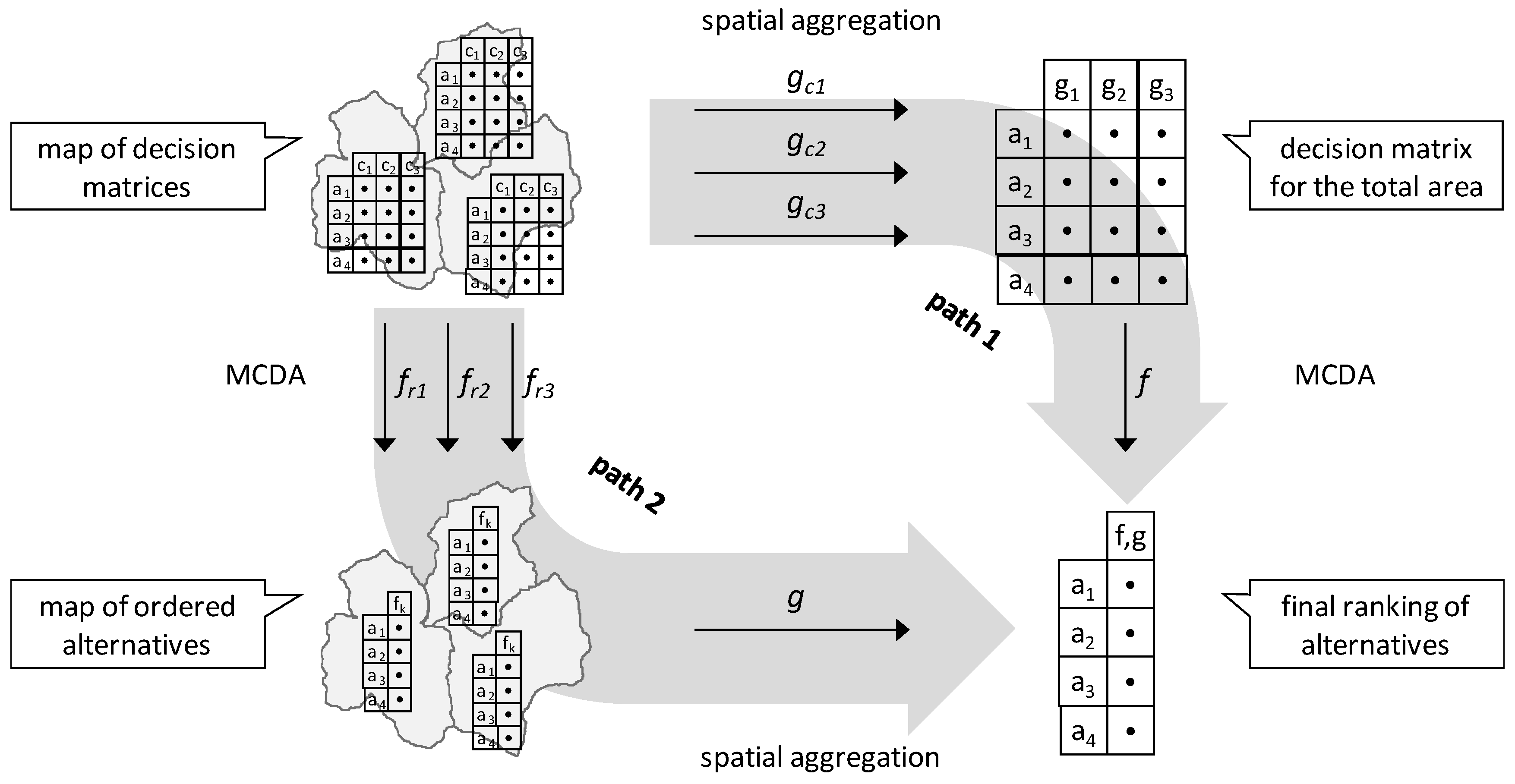
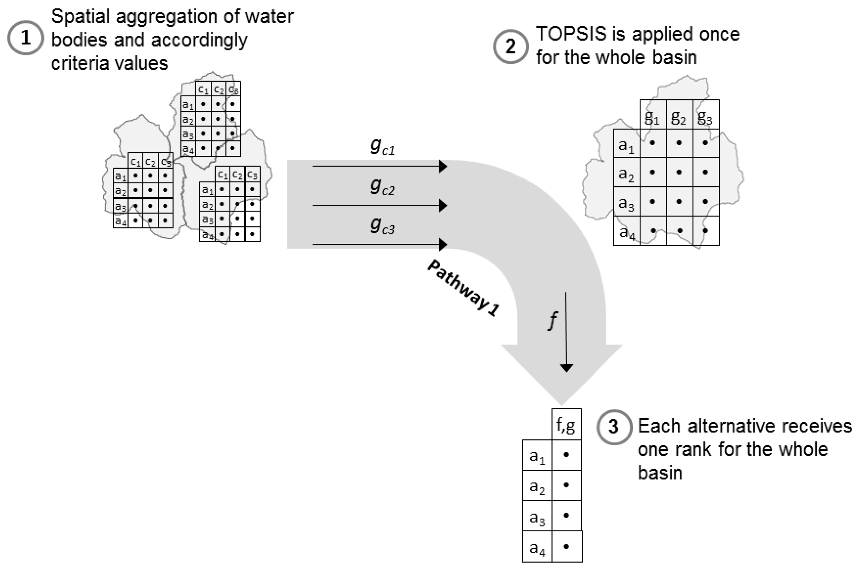
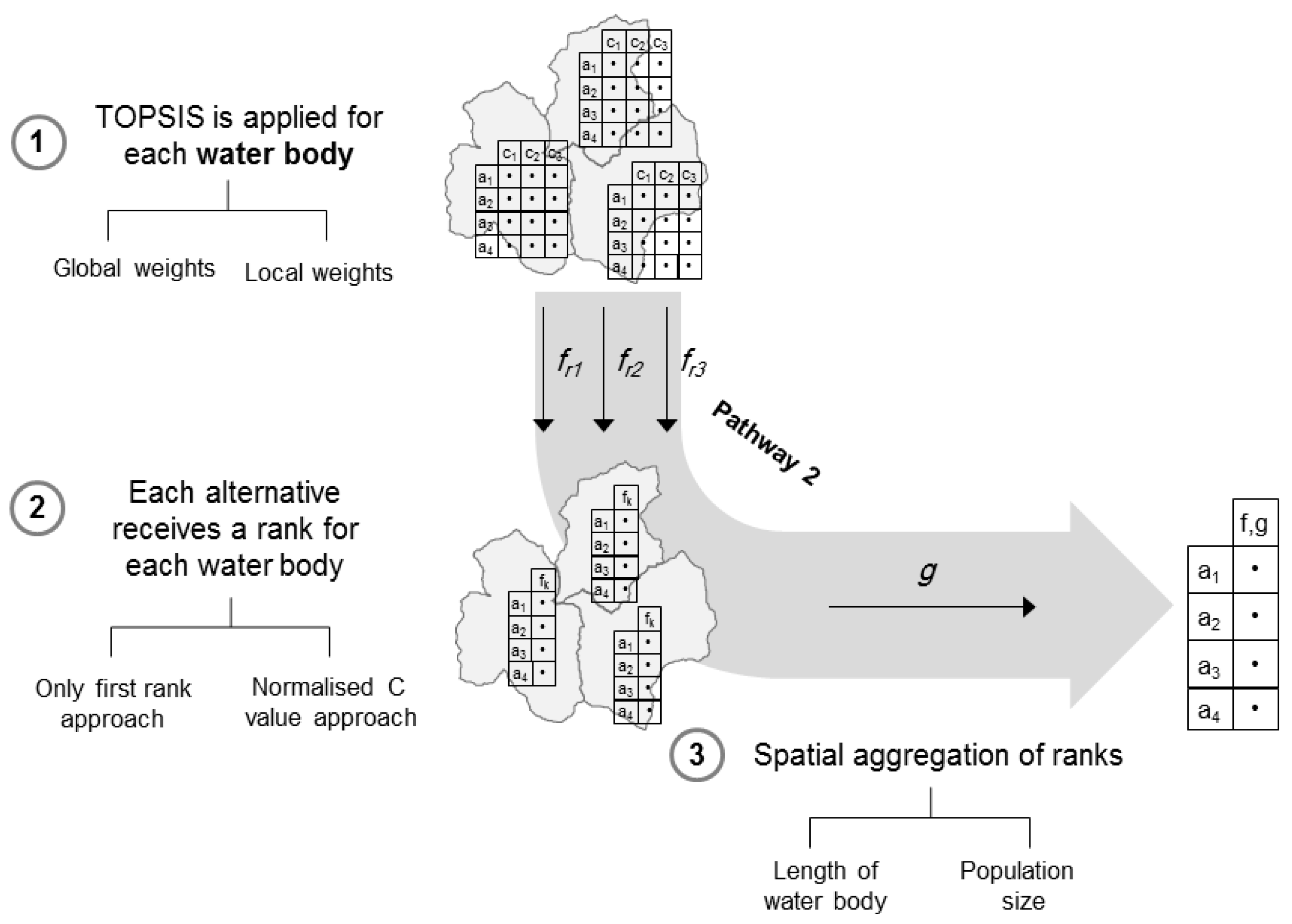
Spatial MCDA problems can be solved via two different aggregation pathways [6] (Figure 1), where the main difference is the order in which MCDA and GIS are applied. Pathway (1) starts with spatial aggregation followed by MCDA. The decision analysis is done for the entire area of interest after removing spatial patterns of the criteria. Pathway (2) starts with applying MCDA in each zone and subsequently performing spatial aggregation of the ranked alternatives. Here, the performance of each individual zone, i.e., the local decision, is regarded more than the spatial patterns of the criteria. A practical example for applying pathways (1) and (2) can be found in Reference [7]. However, the results of applying the two pathways cannot be compared because the final outputs are not the same. Applying pathway (1) in the study resulted in an evaluation map for the performance of each alternative for each criterion; whereas, the application of pathway (2) was done such that scores were weighted by their area size and subsequently aggregated and standardized using the total area [6,7]. For more examples on aggregation, see also References [8,9,10,11,12].
To follow the pathways as explained above, spatial upscaling and downscaling need to be performed. The so-called modifiable areal unit problem (MAUP) was described by Reference [13] based on earlier findings of Reference [14] that analytical results are sensitive towards changes in shape and size of areal units. The MAUP is associated with two effects: the scale effect and the zoning effect. Scale effects are associated with changes in the number and/or size of spatial units whereas, zoning effects are associated with changes in the shape of spatial units (the latter is not considered further in our paper). There are a number of methods proposed to investigate the scale effect, for example carrying out a sensitivity analysis of the MCDA results obtained across different spatial scales, and accordingly identifying the most appropriate spatial scale for the MCDA problem being considered [5,15]. Another method is to consider intra- and inter-relationships of the system at various scales, where for example “objectives of stakeholders at one scale can be included as constraints for optimization at other scales” [5]. However, the literature review suggests that thus far there has been no systematic method particularly tailored to addressing the MAUP [16]. Nevertheless, the range of criterion values allows detecting the most appropriate scale for spatial MCDA, where research has demonstrated that the increase in criterion range becomes negligible at high spatial resolutions [5]. The authors suggest that “the ‘threshold’ point, beyond which there is no significant increase of the range value, can be used for identifying the appropriate scale of analysis,” and can be used for decision making. For more information about the MAUP and some case studies, see also References [17,18,19].
Spatial criteria aggregation also drew attention to spatial compensation and spatial equity considerations. Spatial compensation is “a local deterioration that goes unnoticed because it is compensated by an improvement in another spatial location (or vice versa)”. Spatial equity is a reflection of “the spatial extent underlying summarized criteria” which can be either spatially confined, or can cover a broader spatial scale. Some suggestions to address spatial compensation and spatial equity include adding more criteria to the MCDA problem, or using maps and graphical presentation to allow the recognition of spatial trends [11].
In river basin management, the described spatial compensation during the aggregation of multi-criteria decision alternatives has not yet been well investigated, even though many applications of MCDA have been published. In this paper, we analyze spatial compensation effects by aggregating measures for the improvement of water quality from the local scale to basin scale. We apply the technique for order of preference by similarity to ideal solution (TOPSIS) method, which is an example for distance-based MCDA tools, and which has been applied in many studies related with water resources management. We apply TOPSIS in the context of selecting a River Basin Management Plan (RBMP), using data for the Werra River Basin acquired through a research project carried out from 2002 to 2005 (Integrated River Basin Management for the Werra River, hereinafter referred to as IRBM-W). The IRBM-W was carried out by an interdisciplinary research group with the purpose of developing an integrated framework to achieve the “good ecological status” of the Werra River by the year 2015, as stipulated in the European Water Framework Directive (WFD) [20]. The research objectives of this paper are the following:
- Test the hypothesis that different spatial aggregation pathways (see Figure 1) result in different ranking results;
- For each aggregation pathway, we investigate the scaling effect within the context of selecting an integrated river basin management strategy. We perform this investigation on three different spatial scales: the water body, sub-catchment, and river basin scales;
- As means of reflecting spatial variations onto criteria ranges, we further investigate the effect of applying the Range Sensitivity Principle (RSP) within the water body and sub-catchment scales;
- To allow the comparison of the results for the two pathways, we propose two approaches to aggregate rankings for the entire basin: (1) only using the non-dominated decision alternatives, (2) using the performance values of all alternatives. In using the latter, we aim to reduce spatial compensation across different scales.
2. Materials and Methods
2.1. The Werra Integrated River Basin Management Project
The WFD, which entered into force in 2000, defines a general framework for integrated river basin management within the European Union (EU), aiming to reach a “good status” of water bodies by 2015. Boeuf and Fritsch [21] assessed the implementation of the WFD within the EU in the context of research efforts carried out for this purpose. The assessment indicated that water planning carried out at a hydrological scale rather than an administrative one is an institutional novelty introduced through the Directive. A number of definitions for scale can be found in Article (2) of the WFD including but not limited to: “a body of surface water” (Articles 2–10), “river basin” (Articles 2–13), “sub-basin” (Articles 2–14), and “River Basin District” (RBD) (Articles 2–15). The latter includes one or more adjacent river basins and is stated as “the main unit for management of river basins.” However, the authors [21] report that a larger number of studies covered single basins rather than the whole RBD. Some of the reasons to which this can be attributed include the impracticability of this level and the possible conflict of RBDs with administrative boundaries indicating that “important planning activities are carried out at basin level” [22]. The WFD requires that member states prepare RBMPs and more detailed programs for each RBD within their territories (Article 13).
The Werra River basin is located in Germany and falls within the administrative boundaries of four federal states: Thuringia, Hesse, Lower Saxony, and Bavaria. It covers a total area of 5498 km2 and is situated in the upper part of the Weser River Basin. The land cover is mostly agriculture (52%) and forests (43%), not showing a distinct regional pattern except the Nesse sub-basin (dominated by agriculture) and the southeastern part of the catchment (dominated by the Thuringian Forest middle mountains). The climate is humid with annual average rainfall between 600 mm in the lower lands and 1200 mm in the middle mountains. The hydrological flow regime is pluvial-nival. In 2002, an interdisciplinary research group was commissioned to carry out the IRBM-W project. One of the project’s main objectives was to examine and develop methods for the implementation of the WFD, and set-up an integrated pilot RBMP for the Werra River basin [20].
The water quality of the Werra River and its main tributaries was deteriorated by nutrients from non-point as well as point sources of pollution [23,24]. The IRBM-W focused on nitrate and phosphate for assessing river pollution. Non-point sources of pollution were attributed to agricultural activities; whereas, point sources of pollution originated from wastewater treatment plants, storm water retention networks, and unconnected settlements. Another contributor to the deterioration of water quality (not considered in the IRBM-W) was the potash mining industry causing an increase in the salt load of the river [25]. Further details on the project can be found in References [20,26,27]. We used results from the eco-hydrological catchment model as presented in Reference [24].
The IRBM-W activities were carried out on three functional scales as follows:
- Water body—Where the ecological assessment according to the WFD was performed and all IRBM-W measures were planned. The Werra River and its main tributaries were segmented into 41 water bodies according to the EU typology, with an area of a few km2 to up to 1036 km2.
- Sub-catchment—Represents hydrological catchments of the main tributaries (area of 157 km2 to 1511 km2). We also used this scale for representing regions of different land use, water resources management problems, and stakeholder attitudes, as the Werra basin was politically and economically divided into a western and eastern part by the inner German border until 1990.
- River basin (also referred to as basin or catchment)—The Werra River is a sub-basin of the Weser River for which the RBMP was developed in practice.
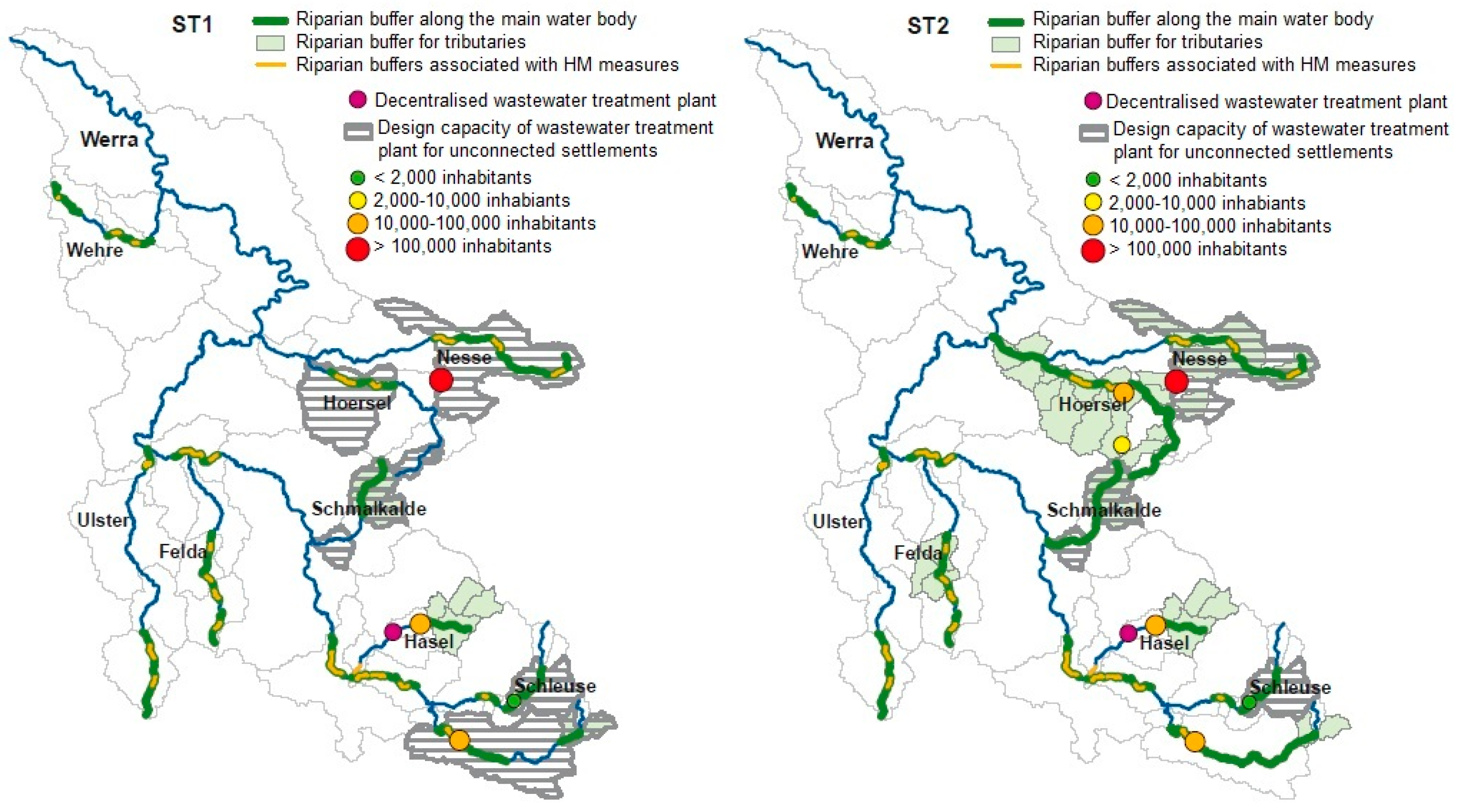
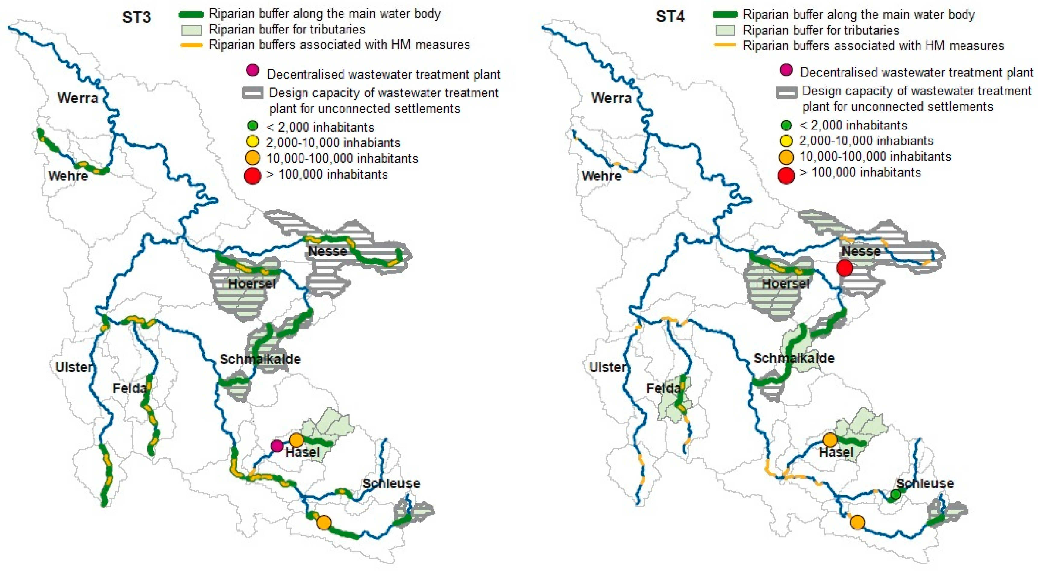
The final IRBM-W was proposed for the entire river basin, containing measures (1) to improve river hydromorphology, (2) to reduce non-point emissions, and (3) to reduce emissions from point sources. Four alternative basin strategies (hereinafter denoted “ST”) were formed from combinations of these various measures for each water body (Figure 2). These strategies comprised of the following approaches based on expert knowledge:
- ST1—Reduce point and then non-point sources of pollution
- ST2—Reduce non-point then point sources of pollution
- ST3—A polluter-oriented distribution of measures
- ST4—Most cost-efficient allocation of measures
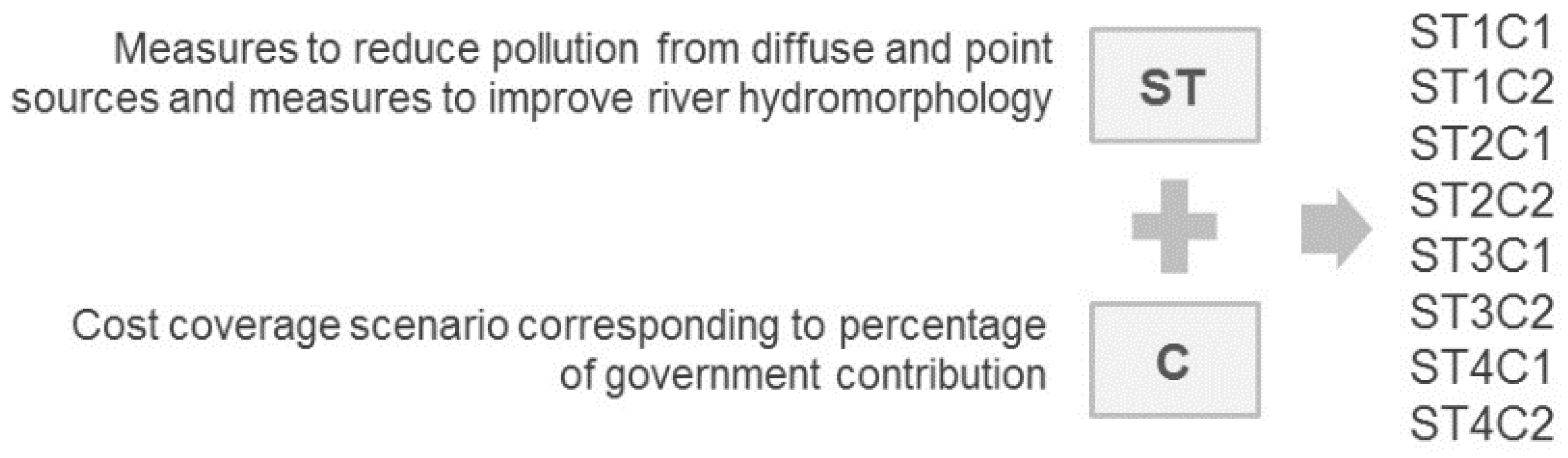
In all strategies, measures for improving the hydromorphological conditions of the water bodies, and measures for reducing non-point phosphorus from soil erosion are included [20,27]. The spatial distribution of the measures proposed for each of the four strategies is shown in Figure 3. Two cost coverage scenarios were considered. In the first scenario (“C1”), however, private entities/persons bear costs associated with the reduction of point source phosphorous and non-point sources of nitrogen. Whereas, in the second scenario (“C2”), the government fully bears the costs to reduce non-point nitrogen and 65% of the costs to reduce point source phosphorous. These two cost coverage scenarios were then considered for each of the ST strategies, finally resulting in eight decision alternatives: ST1C1, ST2C2, ST2C1, ST2C2, ST3C1, ST3C2, ST4C1, and ST4C2 (Figure 2).
The eight decision alternatives were evaluated for the entire Werra river basin with reference to three quantitative evaluation criteria: cost of implementation, ecological and recreational benefits, and stakeholder cooperation [27]. These criteria were selected to represent the three main dimensions of integrated water resources management, namely ecology, economy, and equity (cultural aspects were not accounted for). The three criteria were calculated as independent without double counting. However, implicit relationships exist, e.g., more costs allow better environmental protection and public coverage of costs produces more cooperation than individual cost coverage. Overall, the problem was treated as a multi-criteria decision problem, where costs are expressed in monetary units, ecological benefit is monetized, and cooperation is an index.
Cost estimates were developed based on comparable studies and expert opinion. The costs for the reduction of non-point sources of nutrient emissions were calculated with an agricultural economic model based on regional statistical data [27].
The benefits considered the improvement of ecological functions and recreational opportunities estimated in monetary units using the Total Economic Value (TEV) framework, and applying the Benefit Transfer Method (BTM) [27]. A primary valuation study for the restoration of the Elbe River served as a reference for the benefit transfer for the Werra River [28]. Next to the ecological and recreational benefits associated with the IRBM-W, the “super-additive benefits for developing the whole basin into a good ecological status” were also considered [27]. With this as a backdrop, different value functions were assumed for ecological benefits compared to the recreational benefits. A decreasing marginal benefit curve was assumed to be the utility function for ecological benefits with a degression rate of 1%, and an increasing linear value function was assumed for the recreational benefits. Both monetary criteria were discounted to the year 2025 using 2005 as the reference year and an interest rate of 3%.
To account for the potential support by regional stakeholders during the implementation of the IRBM-W, a cooperation index was developed. The cooperation index was determined by four factors: (1) the degree of being affected by potential measures derived from GIS analysis; (2) the acceptance of the potential measures obtained by a stakeholder survey based on a previous stakeholder analysis; (3) the relative importance of the affected uses in the region according to census data; and (4) the implications of the cost coverage scenario [27]. The cooperation index was calculated on an ordinal scale to provide a quantitative criterion for social/stakeholder acceptance into the decision-making process. A higher cooperation index indicates greater stakeholder cooperation and acceptance for the decision alternative. As an illustrative example, of the two cost coverage scenarios considered, higher cooperation indices were found for the C2 scenario where the government bears most of the costs. Different from public participation, the stakeholder survey and the subsequent computation of the cooperation index aim at representing the interests of all stakeholders in the decision process in a balanced way, but the index was not designed to support a participatory, learning based decision process, where the MCDA would have to be developed differently.
For our research, we use the input data acquired for the IRBM-W, and related considerations essential to achieve Integrated Water Resources Management (IWRM) within the basin. However, we modified the calculation of the cooperation index as follows: (1) rescale by adding +8.5 in order to have only positive values and (2) perform aggregation weighted by population in each water body as opposed to the arithmetic mean used in the original project.
2.2. MCDA with TOPSIS
The TOPSIS [29] is one of many MCDA tools which have been used for a number of applications including water resources management [30,31,32]. The TOPSIS defines the best alternative as the one, which is simultaneously closest to the ideal point and farthest away from the negative ideal point (nadir). The separation measures (from ideal point) and (from nadir) are raised to the power of 0.5 (i.e., p = 2) by using the Euclidian distance (see Equations (1)–(6)). However, different distances can also be considered depending on the value of the p-parameter used. Normally, the p-parameter is a value between 1, 2, and , and “reflects the importance of the maximal deviation from the ideal point” [33]. When p = 2, “each deviation is accounted for in direct proportion to its size, [implying] partial compensation between criteria” [4,5]. For more details on the p-parameter see Reference [34].
The equations as proposed by Reference [21] include the following steps:
Step 1: Construct the normalized decision matrix, which transforms various attribute dimensions into non-dimensional, thus allowing their comparison. Vector normalization is used. By the end of this step, each attribute has the same vector.
where is an element of the normalized decision matrix, is the numerical outcome of the ith alternative for the jth criterion, and m is the number of alternatives.
Step 2: Construct the weighted normalized decision matrix. A set of weights assigned by the decision maker is included in the decision matrix in this step. The weights can express the relative importance of the criteria for the decision maker. These should not be confused with values assigned for the criteria, but their impact on the MCDA results is crucial because it can add a subjective influence on the outcome. The matrix is calculated by multiplying each column (v) of the matrix R (for ) with its associated weight (w).
Step 3: Determine ideal and negative ideal/nadir solutions
where J and J′ are associated to criteria values preferably maximized (e.g., benefit) or minimized (e.g., cost) respectively.
A* = {(maxi vij | j∈J), (minj vij | j∈J′) | i = 1, 2,…, m} = {v1*, v2*, … vj*, … vn*}
Step 4: Calculate the separation measure for n-dimensional Euclidean distance
Step 5: Calculate the relative closeness (C) to the ideal solution
Ai is closer to A* as approaches to 1.
Step 6: Rank the preference order in accordance to .
2.3. Pathways for Aggregation in Spatial MCDA
The RBMPs are proposed at the basin scale in IRBM-W. However, the best alternative for the entire basin is not necessarily the best alternative for each smaller unit (here: water body, sub-catchment). Therefore, in the context of our paper we evaluate the two pathways proposed for aggregation (see Section 1 and Figure 1).
While following pathway (1), we performed spatial aggregation of the water bodies and their respective criteria values to acquire overall values for the entire basin. Cost and benefit values for all water bodies are summed up and cooperation values were averaged. Subsequently, we applied TOPSIS only once using the overall values resulting in one rank for each alternative. This pathway is seen as a top-down approach for decision making because spatial variations in criteria values are not adequately reflected in the decision making problem, and spatial compensation is allowed.
Through pathway (2), we aimed to limit spatial compensation by ranking the alternatives for each smaller spatial unit, and subsequently aggregating the ranks. To do so, we applied TOPSIS for each water body (or sub-catchment). To aggregate the ranks, we used two different weights: the length of water body (where we emphasize the ecological importance of the decision alternative), or the local population size (where we emphasize the social implications of the decision alternative). We view this approach as bottom-up decision making because we use the performance of each decision alternative (represented by its relative rank) for each smaller spatial unit to identify the “best” alternative for the entire basin.
Although the application of pathway (2) was straight forward for upscaling from a water body to a basin scale, we found this not to be strictly the case for sub-catchments. In the latter, we followed a three-step approach. The first step required spatial aggregation for water bodies to acquire aggregated criteria values for each sub-catchment (e.g., the value of the cost criterion for sub-catchment Nesse is the sum of the cost criterion for water bodies Nesse_1 and Nesse_2 of which it consists). In the second step, we applied TOPSIS for each sub-catchment, and in the third step, we aggregated the resulting ranks. Thus, the sub-catchment scale combines both pathways (1) and (2), and as such is a combination of a top-down and bottom-up approach.
2.4. Local Criteria Weights by Using the Range-Sensitivity Principle
Spatially referenced criteria can be weighted globally or locally (using spatially explicit methods) [5,35]. Thus, in addition to reflecting stakeholder preferences, criteria weighing can also account for differences in the range of each evaluation criterion [36]. Global criteria weighing assumes spatial homogeneity of preferences by assigning a single weight to each criterion for the entire area [5]. Global criteria weights could be determined empirically to assign impartial importance to all criteria (representing ecological, economic, and social aspects in IRBM-W). However, there was no such attempt done in our study, so we used equal values for the global weights as the default. Since homogeneity is realistically not the case, we applied a method for the calculation of local criteria in parallel (Figure 6).
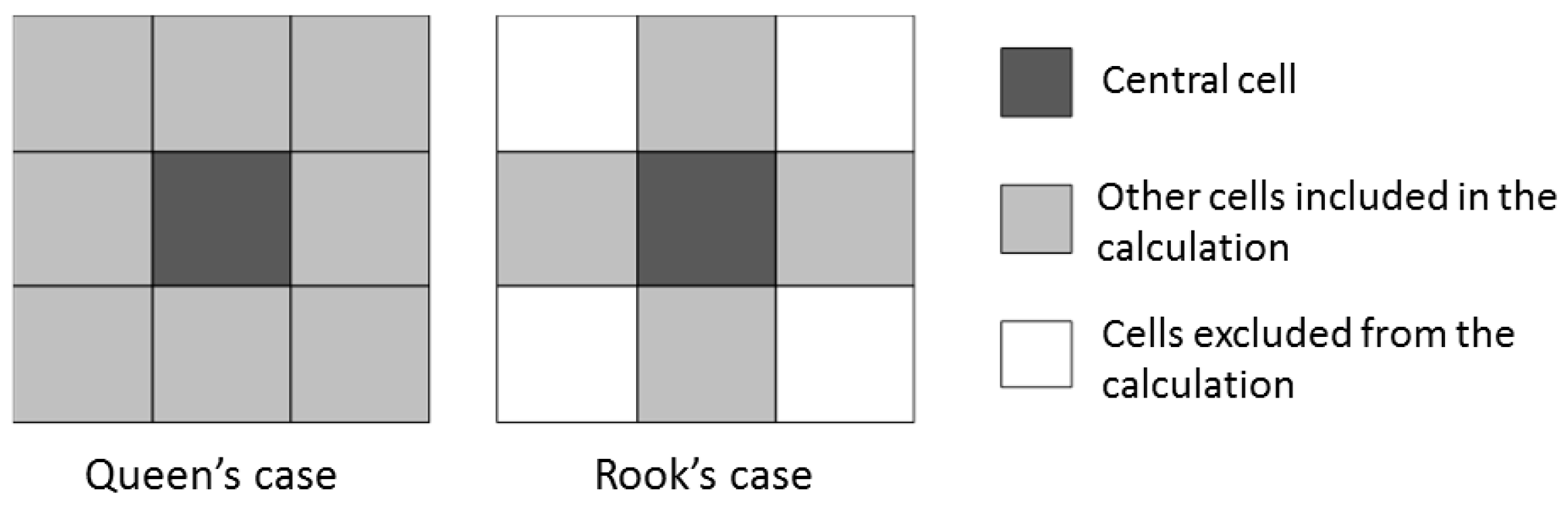
Local/spatially-explicit criteria weighing methods consider spatial heterogeneity of the criteria, and thus, identify local criteria weights for a given location based on its neighborhood. A local neighborhood “q” can be defined using methods such as shared boundary or distance-based methods [35]. Two common shared boundary methods are the Queen’s and Rook’s neighborhoods. Queen’s neighborhood method considers cells sharing at least one point to be neighbors whereas, in Rook’s case a minimum of two shared points are needed for a neighbor [37] (Figure 7).
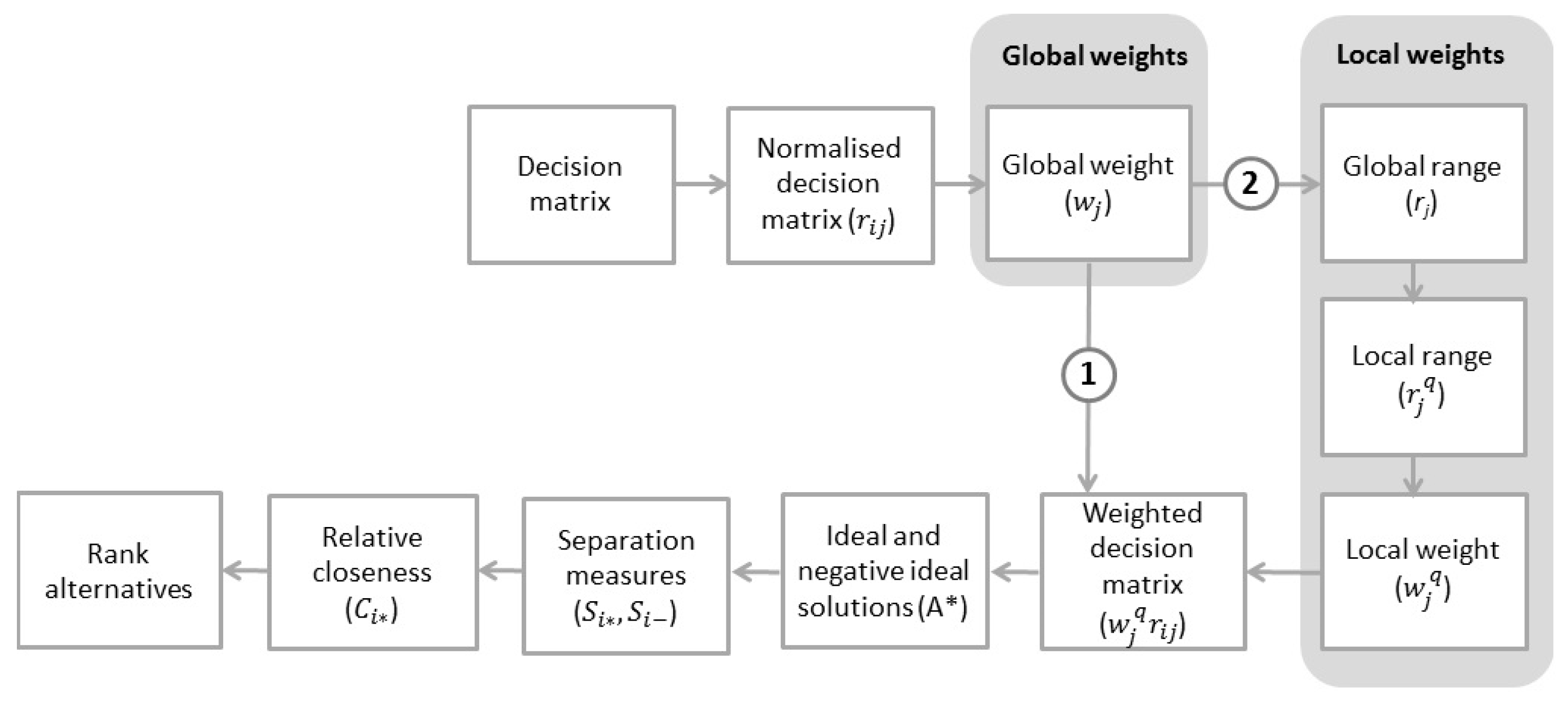
Local weights can be estimated using the range-sensitivity principle (RSP) [35,38,39]. “The RSP suggests that, other things being equal, the greater the range of values for the k-th criterion, the greater the weight wk that should be assigned to that criterion” [35]. Note that, for the purposes of consistency throughout our paper, the k corresponding to each criterion is denoted j and consequently the weight is denoted wj hereinafter. The RSP tailors the relative importance (weight) of each criterion to a given location. These local criteria weights are computed as a function of the global weights, the global range of criteria values, and a local range of criteria values for a specific neighborhood.
Step 1: Identification of the global range and local range
where and and are the maximum and minimum values of the jth criterion within globally or locally for the qth neighborhood, respectively [27].
To identify the within the context of our research for the IRBM-W, we consider the global maximum and minimum values for each criterion across all alternatives and all water bodies or sub-catchments (depending on the spatial scale under consideration). Subsequently, we normalize for each water body or sub-catchment against the whole basin to obtain comparable values.
To identify we apply Queen’s case contingency to identify the neighbors for each water body or sub-catchment. We then calculate the local range considering the maximum and minimum values for each criterion within each spatial unit (water body or sub-catchment) and its neighbors. We then normalize local ranges against the whole basin.
Step 2: Calculate the local criteria weight
Upon identifying the global range and local range (), and having the global criteria weights, we calculate the local criteria weights. Within the context of our research, we calculate the value for each jth criterion and subsequently divide by for all three criteria. In doing so, we obtain the local criteria weight for each criterion considering its local criteria range values.
where is the local weight for the jth criterion in the qth neighborhood, is the global weight of the jth criterion, is the global criterion range and is the local criterion range [35,38].
Here, we draw attention that in 13 of the 41 water bodies, all eight alternatives received equal ranking, i.e., there was no preference for any alternative over the other. Therefore, applying TOPSIS for these 13 water bodies was not possible for mathematical reasons (separation measures and are equal to zero). Nevertheless, although we do not consider these 13 water bodies further during the aggregation of TOPSIS results for the entire basin, we do consider their criteria ranges when applying the RSP to localize criteria weights. We provide a summary of the framework according to which we apply MCDA in our research in Table 1.
2.5. Aggregation Procedure
We apply TOPSIS for each water body and sub-catchment and subsequently, we obtain a relative closeness value (C, Equation (6)) for each alternative alongside its corresponding rank for each spatial unit, i.e., we obtain 41 ranks for the 41 water bodies, and 10 ranks for the 10 sub-catchments. In this step, we propose two methods for aggregating TOPSIS results for the entire catchment (following pathway 2) based on their rank (relative performance) or based on their relative closeness (absolute performance).
The first rank approach only considers the rank of the non-dominated alternatives at each spatial unit, i.e., we do not consider the TOPSIS relative closeness (C) value but rather the final result (see Equation (6)). Subsequently, we assign the non-dominated alternatives a value of 1, and the dominated alternatives a value of zero. Thus, we do not account for the dominated alternatives as we scale up to the basin level. The non-dominated rank serves as an indicator for the “best” alternative within each water body or sub-catchment regardless of how well or bad it performed in other locations, i.e., we allow for spatial compensation. The rationale behind this approach is to emphasize the choice of decision makers at smaller spatial scales (water bodies or sub-catchments) so their local decisions are the ones further aggregated for the basin scale.
The relative closeness (C) value of TOPSIS is a distance measure to the ideal solution (see Equation (6)). Using the C value for rank aggregation during upscaling accounts for the performance of non-dominated as well as dominated alternatives. Therefore, in this case the aggregated rank for the basin scale is indicative of each alternative’s overall performance considering all spatial units. For example, if the alternative ST1C1 is considered the best for water body 1, and the worst for water body 10, the aggregated rank of ST1C1 at the basin scale considers both these results and not only the result for water body 1. In principle, considering the overall performance of each alternative reduces spatial compensation (see Section 1). Using this approach, decision makers can relate the local decisions to the global context. However, the C values we obtain from applying TOPSIS within each spatial unit differs depending on the criteria ranges within this unit. Therefore, the C values are not comparable between various spatial units. Thus, we normalize the C value for each water body or sub-catchment against the sum of all C values for the entire basin for all alternatives considered in the decision space. We perform such normalization twice; once considering the C values, we obtain from using global criteria weights, and once considering the C values, we obtain from using local criteria weights.
Decision alternatives need to be aggregated further to the river basin scale. To do so, we propose two weighing methods for the aggregation of alternatives while upscaling from the water body or sub-catchment scale to the entire basin: (1) the length of water body and (2) the population size. In defining different weighing options for aggregating TOPSIS results, we can accommodate the preference of the decision makers, where the length of water body option allows the decision maker to place more emphasis on ecological considerations, whereas using the population size, he/she places more emphasis on the socio-economic considerations and stakeholder buy-in.
Using the first rank approach, we assign the non-dominated alternatives at each water body or sub-catchment a value corresponding to its length of water body, or its population size. In the final step, we sum up all the values for each alternative for the entire basin, and accordingly, we rank the alternatives descending where the alternative receiving a higher sum receives a higher rank.
3. Results
In total, we computed 17 rankings of the eight alternatives by the combined application of GIS aggregation and TOPSIS. One (indicated in grey in Figure 8 and Figure 9) is following pathway 1, 16 are following pathway 2 (Figure 6), from which eight apply the “first rank” approach for the spatial aggregation of MCDA results using the ranks, and eight follow the “normalized C value” approach using the distance measure of the MCDA. In this section, we compare the results with reference to the following points:
- Stability of the final aggregated ranking for the non-dominated alternative/s—we compared alternatives that ranked as non-dominated after aggregation for the whole basin
- Stability of the final aggregated ranking for the dominated alternatives—We compared the dominated alternatives after aggregation for the whole basin. By stability of rankings here, we refer to rank reversal among the dominated alternatives. For example: rank reversal takes place when an alternative receives a rank of 2 when applying a given method (e.g., using global weights), and a rank of 4 when applying another method (e.g., using local weights). In this case, the rankings are “less stable” because we note a change in the ranking
- Extent of rank reversal/variation—We linked the concept of stability of ranking with the “extent” to which rank reversal takes place. Taking the same example above, we report an extent of rank reversal of ±2 ranks. Therefore, the greater the extent of rank reversal, the greater the difference between the rankings of alternatives resulting from the application of different methods; for example, ±4 ranks have a higher extent of rank reversals than ±2 ranks
- Discriminative power of rankings of alternatives—The discriminative power of rankings refers to the number of alternatives receiving the same rank; a high discriminative power means that no two (or more) alternatives receive the same rank
In our results, a higher stability of rankings among non-dominated and dominated strategies, and in comparison to rankings at the basin scale results, is a desirable property. By definition, this also corresponds to a lower extent of rank reversal. Our reasoning entails that, the more stable the rankings, the more reliable is the final decision as it is less prone to changes associated to spatial scaling and the corresponding change in decision inputs. We deem a higher discriminative power a desirable property as well because it indicates a clear relative preference among decision alternatives.
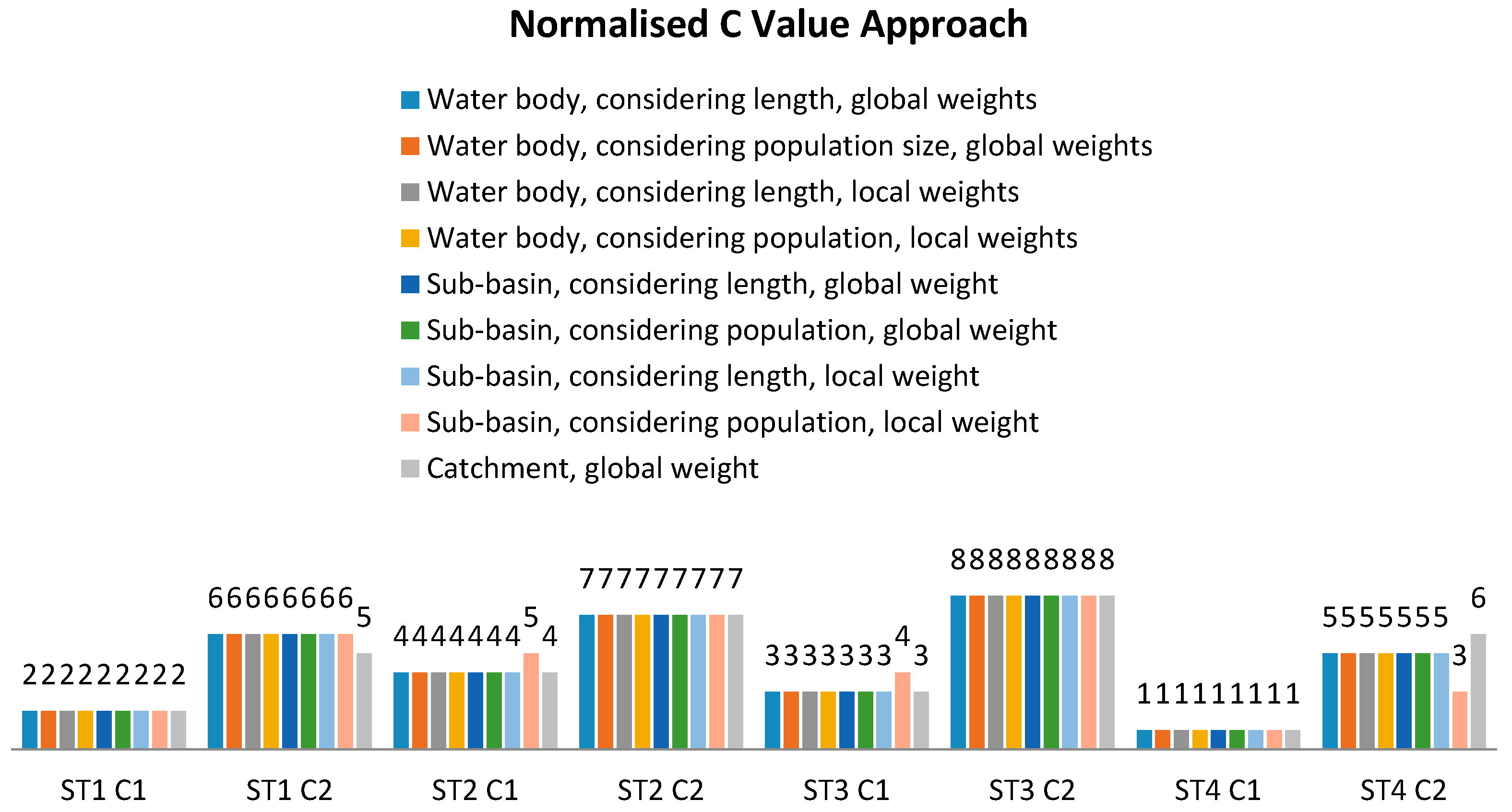
3.1. Normalized TOPSIS Relative Closeness (C) Value Approach
The normalized TOPSIS C value approach results in alternative ST4C1 being non-dominated (rank 1 for all variations of the aggregation procedure, Figure 8). Using the full performance information of the MCDA method (here computed from a distance measure) generally shows a high consistency of rankings among the alternatives. The results from this approach (as shown by the eight colored bars on the left for each strategy in Figure 8) are very similar to those, which we obtain from the aggregation at basin scale (right bar for each alternative shown in grey color in Figure 8). This gives a proof that the two aggregation pathways (Figure 5, Figure 6 and Figure 7) lead to similar ranking results. Thus, the solution of the decision problem is robust against the method of spatial aggregation.
The introduction of local weights at the sub-catchment scale and using the population size for weighing during aggregation, however, results in rank reversal with an extent of ±1 to ±2 (and ±3 when compared to the basin scale).
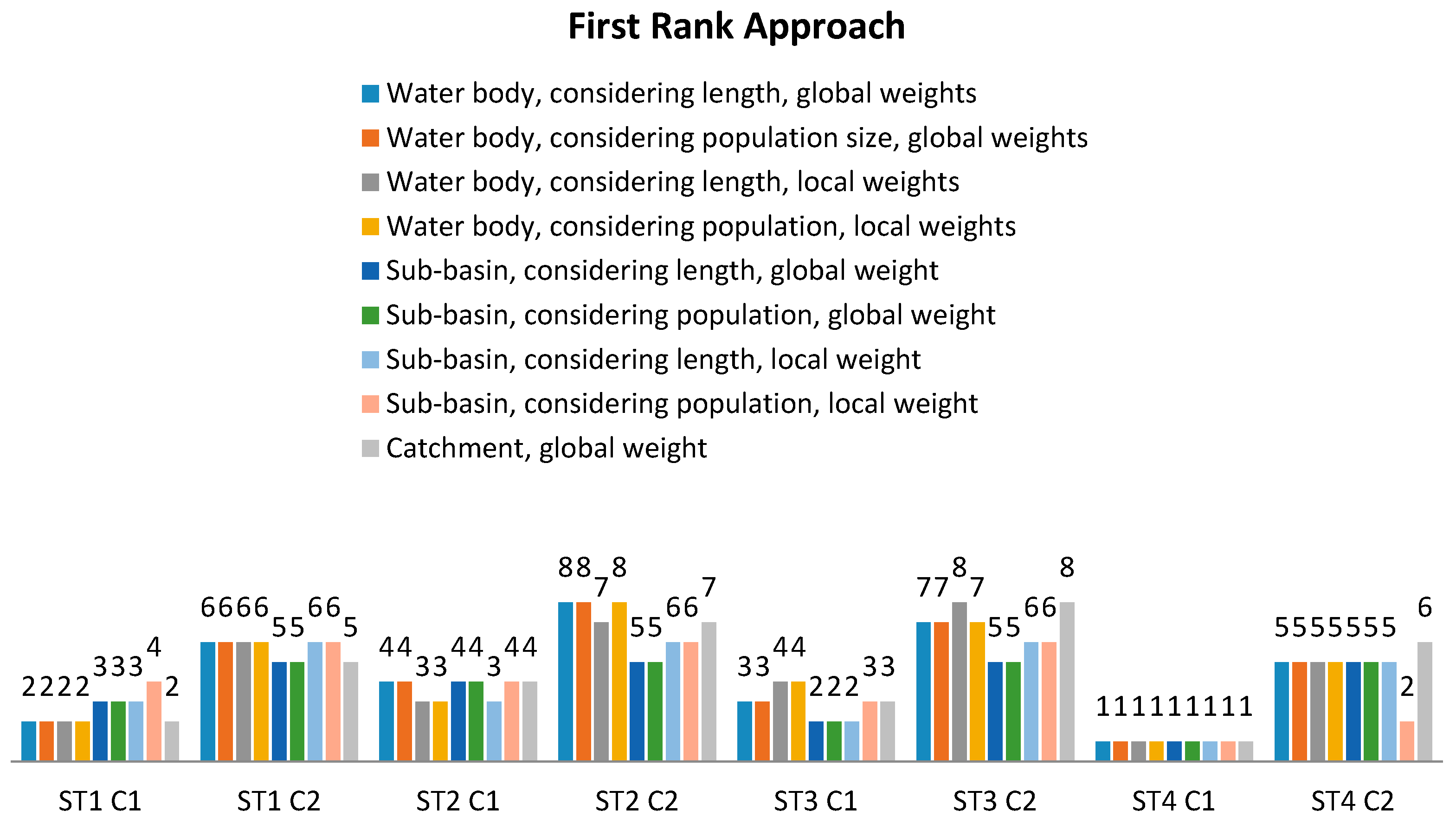
3.2. First Rank Approach
Our results suggest that pathways (1) and (2) tend to produce more similar results when using the water body scale compared to the results obtained at the sub-catchment scale (in Figure 9, the four bars on the left for each alternative are similar and closer to the basin scale aggregation shown by the grey bar on the right). Furthermore, all the methods we consider using the first rank approach (i.e., the three spatial scales, using global and local criteria weights, and applying weights for the length of water body and population size) lead to the same alternative (ST4C1) being the non-dominated. We note the highest stability of rankings for alternatives ST1C2 and ST2C1, where the extent of rank reversal is ±1. However, our results show higher rank stability when comparing the water body and basin scales (±1 rank), rather than comparing the sub-catchment and basin scales. In the latter, the extent of rank reversal increases up to ±4 ranks, thus, the sub-catchment scale introduces a higher margin of variation among rankings. The use of local criteria weights at the sub-catchment scale increases the extent of rank reversal from ±1 using global criteria weights, to ±4.
The water body and basin scales show a high discriminative power of rankings, i.e., none of the alternatives receives the same rank as any other. The sub-catchment scale, on the other hand, shows a lower discriminative power where two (or more) alternatives receive the same ranking.
Furthermore, the use of local criteria weights at the water body scale does not decrease the discriminative power of alternatives, nor does it increase it at a sub-catchment scale. In contrast, on a sub-catchment scale, the use of local criteria weights decreases the discriminative power (Figure 9).
3.3. Other Findings
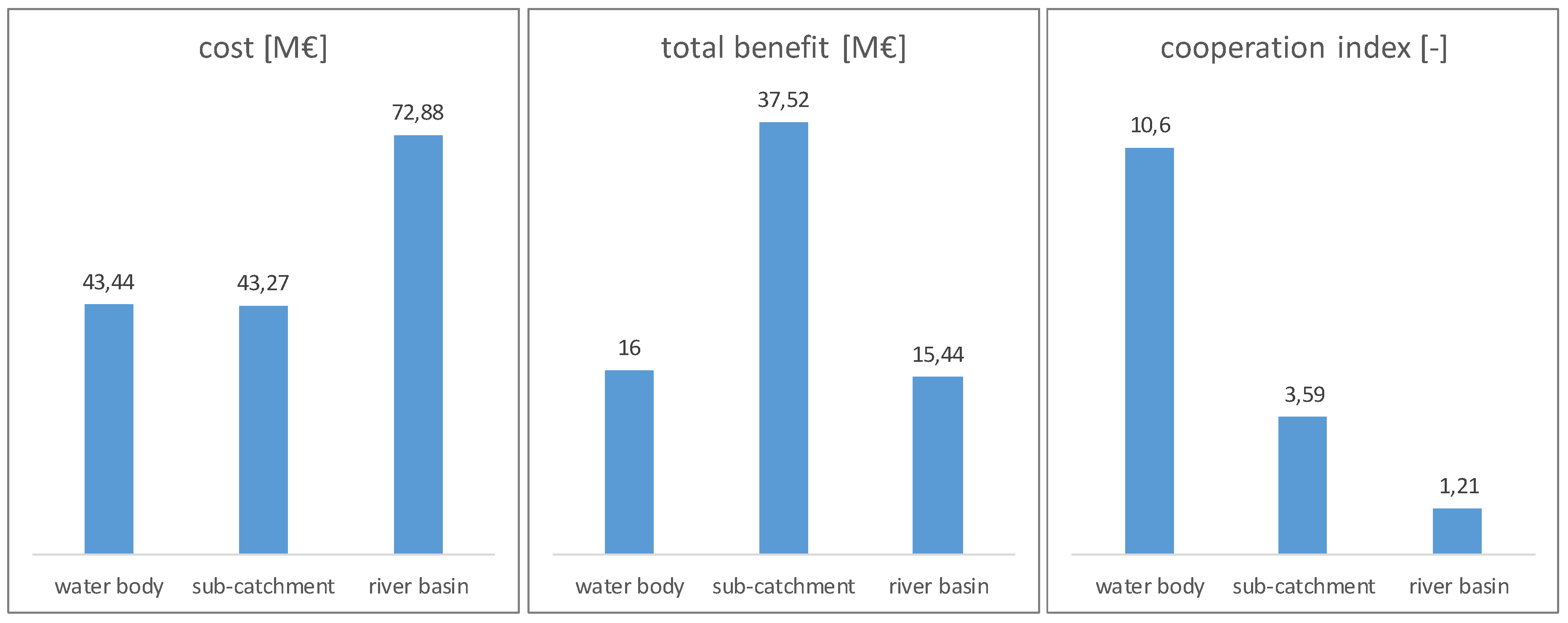
Beyond the direct objectives of our research, we also present our findings regarding criteria ranges corresponding to a decrease in spatial resolution. We calculate these ranges based on the maximum and minimum criteria values for all the alternatives across all water bodies, sub-catchments, and the aggregated values for the entire basin.
Our results show that the costs criterion’s maximum range falls at the lowest resolution (the basin scale). It also demonstrates little change after a “threshold” of 10 spatial units (corresponding to the sub-catchment scale). For the benefits criterion, on the other hand, we note the maximum range at the scale of 10 spatial units (sub-catchment). The cooperation index shows the maximum range at the highest resolution of 41 spatial units (water body scale) (Figure 10).
4. Discussion
Applying the RSP to localize criteria weights for each neighborhood defined using Queen’s case contingency resulted in a change in the criteria weights. In neighborhoods, where a certain criterion shows a range of zero, i.e., all alternatives receive an equal value, the corresponding weight was also zero. We find this to be a logical output indicating that this criterion is “unimportant” within this local neighborhood.
The results demonstrate that in all cases ST4C1 ranks as the “best”. The alternative ST4 constitutes of expert-based optimization of the overall river basin management plan. Thus, the results suggest that, from a river basin management perspective, the “best” alternative for the entire basin is one, which considers it in its entirety considering an economic optimization of the measures. Furthermore, C1 is the cost coverage alternative where the government and private entities/persons share the costs for implementing the proposed measures [20]. Thus, the results also suggest that the lower cost alternative (from the government’s perspective, i.e., the decision maker) is favored in terms of funding. Here, we draw attention that the stakeholders’ cooperation has been factored into the decision through the cooperation index.
Furthermore, when allowing for spatial compensation (i.e., using the first rank approach), we note less stability among the ranking of dominated alternatives. Thus, any change in the spatial scale, criteria weights, and/or weighing method for aggregation during upscaling brings about rank reversal. On the other hand, when we limit spatial compensation (i.e., apply the normalized TOPSIS C value approach), we note higher stability in rankings and a higher discriminative power too. However, a number of points must be regarded while applying the normalized TOPSIS C value approach. First, because the normalization is done against the sum of C values across all spatial units and alternatives, any additional alternatives will change the decision space, and thus, a new decision problem has to be evaluated starting all over again. In that sense, the alternatives become dependent on one another to solve the decision problem because of the normalization. Nevertheless, to eliminate such dependency among decision alternatives, normalization can also be done against a pre-determined C value, which is based on expected maxima of criteria ranges.
On another hand, the maximum ranges we note for the costs and cooperation criteria do not contradict our expectations. The costs criterion is aggregated using summation; thus we find it logical that we note the maximum range at a basin scale. The cooperation index shows the maximum range at the highest resolution of 41 spatial units (water body scale). This we also find logical because, during upscaling, we aggregate the criterion taking weighted averages, and thus, compensation effects are shown by smoothening the results. The maximum range for the benefits criterion, however, contradicts our expectation. Given that the benefits criterion, similar to the cost criterion, is aggregated using summation, we expect the benefits criterion to show the highest range at the basin scale too. Given these variations in the behavior of the evaluation criteria corresponding to a decrease in the spatial scale, we cannot conclusively say which spatial scale is the “most appropriate” for solving the MCDA problem considering all three criteria.
5. Conclusions
Upon applying TOPSIS on different spatial scales, and aggregating the results for the river basin scale, we find that there is no variation in the final non-dominated alternative selected regardless of the different aggregation pathways we follow. However, we do note rank reversal among the dominated alternatives. Furthermore, in comparison to the water body scale, generally the sub-catchment scale seems to be more prone to rank reversal when decision inputs change, e.g., criteria weights or weighing for aggregation of TOPSIS results during upscaling.
Applying the RSP to localize criteria weights for each neighborhood defined using Queen’s case contingency results in a change in the criteria weights. This change, we find, reflects local criteria ranges better than global criteria ranges. However, using the first rank approach shows that both the water body and sub-catchment scales are prone to rank reversal when changing global weights to local weights, whereas this is only the case for the sub-catchment scale when considering population size as the weighing option for aggregation.
The first rank approach allows spatial compensation when compared to the normalized C value approach. Furthermore, the first rank approach, when compared to the normalized TOPSIS C value approach, shows more sensitivity to changing decision inputs demonstrated in a higher extent of rank reversal. Thus, only accounting for local decisions in making decisions at a larger spatial unit is not “stable” and could result in different rankings especially among dominated alternatives. This is especially the case for the sub-catchment scale. However, the normalized C value approach is more stable even when decision inputs are changed.
The normalized C value approach also shows an improvement in the discriminative power of alternatives especially at the sub-catchment scale. Moreover, the two proposed weighing options for aggregating TOPSIS results during upscaling play a greater role in the first rank approach in contrast to the normalized C value approach.
Finally, our results show that the costs, benefits, and cooperation index criteria show highest ranges on a basin, sub-catchment, and water body scales, respectively.
We applied straightforward mathematical concepts and employed simple tools from ArcGIS and Microsoft Excel. Therefore, it is relatively easy for decision makers to apply and reproduce the methods we propose. However, using Microsoft Excel for a large number of spatial units and/or continuously changing decision alternatives becomes laborious, time consuming, and can result in errors. Therefore, we propose using programming tools that are also able to accommodate dynamic systems where additional alternatives can be considered in the decision problem.
Finally, our numerical results are specifically tailored to the IRBM-W case study and the results depend on the input data and the MCDA method used. The modelling of nutrients at the catchment scale is subject to uncertainties from many sources. The definition and the integrated assessment of the eight strategies was assumed as “precise” or “true” input into our procedure, but the criteria have been calculated by imperfect models, which were fed by uncertain data. We just investigated the effects of multi-criteria aggregation of a given dataset and we showed that the pathway and other aspects of spatial MCDA aggregation have an impact on the result. We have chosen TOPSIS for MCDA, because it was used in several water resources decision support systems and because it stands for a well-established group of distance-based MCDA methods. Nevertheless, the results of aggregation can be different if other methods, even of a different class of MCDA tools like outranking methods, are applied with the same input dataset. With our study, we can show the importance of spatial compensation and we want to point out that the application of MCDA in spatial decision support requires such kind of analysis in order to get a more robust overall result. We recommend further research to investigate the transferability of our methods, results, and conclusions to other river basins and other MCDA methods.
Author Contributions
Conceptualization: R.T. and J.D. Data curation: J.D. Methodology: R.T. (for spatial and MCDA aggregation), and J.D., A.D. and J.H. (Werra RBMP. Software: R.T. Supervision: J.D. Validation: J.D. and A.D. Writing–original draft: R.T., J.D. and A.D. Writing–review & editing: R.T. and J.D.
Funding
This research was funded by the German Federal Ministry of Education and Research (Bundesministerium für Bildung und Forschung, BMBF), grant number FKZ 0330211. Deutscher Akademischer Austausch Dienst (DAAD) funded the postgraduate studies of Rania Taha under the EPOS program (Development-Related Postgraduate Courses). The publication of this article was funded by the Open Access Fund of the Leibniz Universität Hannover.
Acknowledgments
This work is based on results of the joint research project “River Basin Management of the Werra River” (principal investigator: Andreas Schumann, Ruhr-Universität Bochum). We thank all partners for their collaborative efforts and for sharing data, knowledge, and results. We are thankful for the constructive comments of the reviewers, which helped to improve our paper.
Conflicts of Interest
The authors declare no conflict of interest.
References
- Hajkowicz, S.; Collins, K. A Review of Multiple Criteria Analysis for Water Resource Planning and Management. Water Res. Manag. 2007, 21, 1553–1566. [Google Scholar] [CrossRef]
- Romero, C.; Rehman, T. Natural resource management and the use of multiple criteria decision-making techniques: A review. Eur. Rev. Agric. Econ. 1987, 14, 61–89. [Google Scholar] [CrossRef]
- Hajkowicz, S. A comparison of multiple criteria analysis and unaided approaches to environmental decision making. Environ. Sci. Policy 2007, 10, 177–184. [Google Scholar] [CrossRef]
- Zeleny, M. Multiple Criteria Decision Making; McGraw-Hill: New York, NY, USA, 1982. [Google Scholar]
- Malczewski, J.; Rinner, C. Multicriteria Decision Analysis in Geographic Information Science; Springer: New York, NY, USA, 2015. [Google Scholar]
- Herwijnen, M.; van Janssen, R. The use of multi-criteria analysis in a spatial context. In Spatial Information and the Environment; Halls, P., Ed.; Taylor and Francis: London, UK, 2001; pp. 259–272. [Google Scholar]
- Janssen, R.; Goosen, H.; Verhoeven, M.L.; Verhoeven, J.T.A.; Omtzigt, A.Q.A.; Maltby, E. Decision support for integrated wetland management. Environ. Model. Softw. 2005, 20, 215–229. [Google Scholar] [CrossRef]
- Yager, R.R. On Ordered Weighted Averaging Aggregation Operators in Multicriteria Decisionmaking. IEEE Trans. Syst. Man Cybern. 1988, 18, 183–190. [Google Scholar] [CrossRef]
- Tkach, R.J.; Simonovic, S. A new approach to multi-criteria decision making in water resources. J. Geogr. Inf. Decis. Anal. 1997, 1, 25–43. [Google Scholar]
- Makropoulos, C.K.; Butler, D. Spatial ordered weighted averaging: Incorporating spatially variable attitude towards risk in spatial multi-criteria decision-making. Environ. Model. Softw. 2006, 21, 69–84. [Google Scholar] [CrossRef]
- Nijssen, D.; Schumann, A.H. Aggregating spatially explicit criteria: Avoiding spatial compensation. Int. J. River Basin Manag. 2014, 12, 87–98. [Google Scholar] [CrossRef]
- Malczewski, J. Ordered weighted averaging with fuzzy quantifiers: GIS-based multicriteria evaluation for land-use suitability analysis. Int. J. Appl. Earth Obs. Geoinf. 2006, 8, 270–277. [Google Scholar] [CrossRef]
- Openshaw, S.; Taylor, P.J. A Million or so Correlation Coefficients: Three Experiments on the Modifiable Areal Unit Problem. In Statistical Applications in the Spatial Sciences; Wrigley, N., Ed.; Pion: London, UK, 1979; pp. 127–144. [Google Scholar]
- Gehlke, C.E.; Biehl, K. Certain Effects of Grouping upon the Size of the Correlation Coefficient in Census Tract Material. J. Am. Stat. Assoc. Suppl. 1934, 29, 169–170. [Google Scholar]
- Marceau, D.J. The Scale Issue in the Social and Natural Sciences. Can. J. Remote Sens. 1999, 25, 347–356. [Google Scholar] [CrossRef]
- McDonnell, R.A. Challenges for Integrated Water Resources Management: How Do We Provide the Knowledge to Support Truly Integrated Thinking? Int. J. Water Resour. Dev. 2008, 24, 131–143. [Google Scholar] [CrossRef] [Green Version]
- Wu, J.; Li, H. Concepts of scale and scaling. In Scaling and Uncertainty Analysis in Ecology: Methods and Applications; Wu, J., Jones, K.B., Li, H., Loucks, O.L., Eds.; Springer: Dordrecht, The Netherlands, 2006; pp. 3–15. [Google Scholar]
- Salmivaara, A.; Porkka, M.; Kummu, M.; Keskinen, M.; Guillaume, J.H.A.; Varis, O. Exploring the Modifiable Areal Unit Problem in Spatial Water Assessments: A Case of Water Shortage in Monsoon Asia. Water 2015, 7, 898–917. [Google Scholar] [CrossRef] [Green Version]
- Lechner, A.M.; Langford, W.T.; Jones, S.D.; Bekessy, S.A.; Gordon, A. Investigating species–environment relationships at multiple scales: Differentiating between intrinsic scale and the modifiable areal unit problem. Ecol. Complex. 2012, 11, 91–102. [Google Scholar] [CrossRef]
- Dietrich, J.; Schumann, A. (Eds.) Werkzeuge für das integrierte Flussgebietsmanagement: Ergebnisse der Fallstudie Werra. In Konzepte für die nachhaltige Entwicklung einer Flusslandschaft Bd. 7; Weissensee-Verlag: Berlin, Germany, 2006. [Google Scholar]
- Boeuf, B.; Fritsch, O. Studying the implementation of the Water Framework Directive in Europe: A meta-analysis of 89 journal articles. Ecol. Soc. 2016, 21, 19. [Google Scholar] [CrossRef]
- Koontz, T.M.; Newig, J. From Planning to Implementation: Top-Down and Bottom-Up Approaches for Collaborative Watershed Management. Policy Stud. J. 2014, 42, 416–442. [Google Scholar] [CrossRef] [Green Version]
- Hirt, U.; Venohr, M.; Kreins, P.; Behrendt, H. Modelling nutrient emissions and the impact of nutrient reduction measures in the Weser river basin, Germany. Water Sci. Technol. 2008, 58, 2251–2258. [Google Scholar] [CrossRef]
- Dietrich, J.; Funke, M. Integrated catchment modelling within a strategic planning and decision making process: Werra case study. Phys. Chem. Earthparts A/B/C 2009, 34, 580–588. [Google Scholar] [CrossRef]
- Bäthe, J.; Coring, E. Biological effects of anthropogenic salt-load on the aquatic Fauna: A synthesis of 17 years of biological survey on the rivers Werra and Weser. Limnologica 2011, 41, 125–133. [Google Scholar] [CrossRef] [Green Version]
- Dietrich, J. Scaling issues in multi-criteria evaluation of combinations of measures for integrated river basin management. Proc. IAHS 2016, 373, 19–24. [Google Scholar] [CrossRef] [Green Version]
- Hirschfeld, J.; Dehnhardt, A.; Dietrich, J. Socioeconomic analysis within an interdisciplinary spatial decision support system for an integrated management of the Werra River Basin. Limnologica 2005, 35, 234–244. [Google Scholar] [CrossRef] [Green Version]
- Meyerhoff, J.; Dehnhardt, A. The European water framework directive and economic valuation of wetlands: The restoration of floodplains along the river Elbe. Eur. Environ. 2007, 17, 18–36. [Google Scholar] [CrossRef]
- Hwang, C.-L.; Yoon, K. Multiple Attribute Decision Making: Methods and Applications: A State-of-the-Art Survey; Springer: Berlin/Heidelberg, Germany, 1981. [Google Scholar]
- Srdjevic, B.; Medeiros, Y.D.P.; Faria, A.S. An objective multi-criteria evaluation of water management scenarios. Water Resour Manag. 2004, 18, 35–54. [Google Scholar] [CrossRef]
- Shih, H.-S.; Shyur, H.-J.; Lee, E.S. An extension of TOPSIS for group decision making. Math. Comput. Model. 2007, 45, 801–813. [Google Scholar] [CrossRef]
- Behzadian, M.; Otaghsara, S.K.; Yazdani, M.; Ignatius, J. A state-of the-art survey of TOPSIS applications. Expert Syst. Appl. 2012, 39, 13051–13069. [Google Scholar] [CrossRef]
- Malczewski, J. GIS and Multicriteria Decision Analysis; John Wiley & Sons: New York, NY, USA, 1999. [Google Scholar]
- Karni, E.; Werczberger, E. The compromise criterion in MCDM: Interpretation and sensitivity to the p parameter. Environ. Plan B 1995, 22, 407–418. [Google Scholar]
- Malczewski, J. Local Weighted Linear Combination. Trans. GIS 2011, 15, 439–455. [Google Scholar] [CrossRef]
- Massam, B.H. Multi-Criteria Decision Making (MCDM) techniques in planning. Prog. Plan. 1988, 30, 1–84. [Google Scholar] [CrossRef]
- Lloyd, C. Spatial Data Analysis—An Introduction for GIS Users; Oxford University Press: Oxford, UK, 2010. [Google Scholar]
- Feick, R.; Hall, B. A method for examining the spatial dimension of multi-criteria weight sensitivity. Int. J. Geogr. Inf. Sci. 2004, 18, 815–840. [Google Scholar] [CrossRef]
- Nitzsch, R.V.; Weber, M. The Effect of Attribute Ranges on Weights in Multiattribute Utility Measurements. Manag. Sci. 1993, 39, 937–943. [Google Scholar] [CrossRef]
Figure 1.
Graphical illustration of the two pathways for spatial multi-criteria aggregation evaluating the relative performance of alternatives based on spatial information (modified from Reference [6]).
Figure 1.
Graphical illustration of the two pathways for spatial multi-criteria aggregation evaluating the relative performance of alternatives based on spatial information (modified from Reference [6]).

Figure 2.
Summary of the proposed decision alternatives for the Integrated River Basin Management for the Werra River (IRBM-W) combining four emission strategies with two cost coverage scenarios.
Figure 2.
Summary of the proposed decision alternatives for the Integrated River Basin Management for the Werra River (IRBM-W) combining four emission strategies with two cost coverage scenarios.

Figure 3.
Measures proposed for the Werra River Basin under each of the four emission strategies in combination with the measures for improving river hydromorphology (ST1 and ST2 from Reference [24], ST3 and ST4 modified from Reference [20]).


Figure 4.
Methodology for pathway (1) considering the basin spatial scale, where we perform spatial aggregation (and accordingly criteria aggregation) as a first step, and subsequently apply TOPSIS to the entire basin.
Figure 4.
Methodology for pathway (1) considering the basin spatial scale, where we perform spatial aggregation (and accordingly criteria aggregation) as a first step, and subsequently apply TOPSIS to the entire basin.

Figure 5.
Methodology for pathway (2) considering the water body spatial scale, where we apply the technique for order of preference by similarity to ideal solution (TOPSIS) to each water body and subsequently aggregate the resulting ranks.
Figure 5.
Methodology for pathway (2) considering the water body spatial scale, where we apply the technique for order of preference by similarity to ideal solution (TOPSIS) to each water body and subsequently aggregate the resulting ranks.

Figure 6.
Graphical representation of the steps for applying TOPSIS using global (route 1) and local criteria weights (route 2).
Figure 6.
Graphical representation of the steps for applying TOPSIS using global (route 1) and local criteria weights (route 2).

Figure 7.
Two methods for defining neighborhood: Queen’s case contiguity (left) and Rook’s case contiguity (right), changed from Reference [30].
Figure 7.
Two methods for defining neighborhood: Queen’s case contiguity (left) and Rook’s case contiguity (right), changed from Reference [30].

Figure 8.
The results from applying TOPSIS on the water body, sub-catchment and basin scales for the different decision inputs we consider. The final rank results obtained at the water body and sub-catchment scale are aggregated using the normalised TOPSIS C value approach.
Figure 8.
The results from applying TOPSIS on the water body, sub-catchment and basin scales for the different decision inputs we consider. The final rank results obtained at the water body and sub-catchment scale are aggregated using the normalised TOPSIS C value approach.

Figure 9.
The results from applying TOPSIS on the water body, sub-catchment, and basin scales for the different decision inputs we consider. The final rank results obtained at the water body and sub-catchment scale are aggregated using the first rank approach.
Figure 9.
The results from applying TOPSIS on the water body, sub-catchment, and basin scales for the different decision inputs we consider. The final rank results obtained at the water body and sub-catchment scale are aggregated using the first rank approach.

Figure 10.
Changes in the cost, total benefit, and cooperation index criteria ranges alongside their corresponding spatial scales: the water body (41 spatial units), sub-catchment (10 spatial units), and river basin (1 spatial unit).
Figure 10.
Changes in the cost, total benefit, and cooperation index criteria ranges alongside their corresponding spatial scales: the water body (41 spatial units), sub-catchment (10 spatial units), and river basin (1 spatial unit).


Table 1.
Summary of the framework according to which we apply MCDA in our research.
| Decision alternatives | ST1C1, ST1C2, ST2C1, ST2C2, ST3C1, ST3C2, ST4C1, ST4C2 |
| Evaluation criteria | Cost of implementation, ecological benefit, cooperation index |
| MCDA method | TOPSIS |
| Measure of separation from ideal and anti-ideal/nadir points | Euclidean distance |
| Ideal and anti-ideal/nadir identification functions | Minimize for costs and maximize for total benefits and cooperation index |
| Global criteria weighing | Equal weights |
| Local criteria weighing method | Range Sensitivity Principle (RSP) |
| Neighborhood determination method | Queen’s case contingency |
© 2019 by the authors. Licensee MDPI, Basel, Switzerland. This article is an open access article distributed under the terms and conditions of the Creative Commons Attribution (CC BY) license (http://creativecommons.org/licenses/by/4.0/).
Share and Cite
MDPI and ACS Style
Taha, R.; Dietrich, J.; Dehnhardt, A.; Hirschfeld, J. Scaling Effects in Spatial Multi-Criteria Decision Aggregation in Integrated River Basin Management. Water 2019, 11, 355. https://doi.org/10.3390/w11020355
AMA Style
Taha R, Dietrich J, Dehnhardt A, Hirschfeld J. Scaling Effects in Spatial Multi-Criteria Decision Aggregation in Integrated River Basin Management. Water. 2019; 11(2):355. https://doi.org/10.3390/w11020355
Chicago/Turabian StyleTaha, Rania, Jörg Dietrich, Alexandra Dehnhardt, and Jesko Hirschfeld. 2019. "Scaling Effects in Spatial Multi-Criteria Decision Aggregation in Integrated River Basin Management" Water 11, no. 2: 355. https://doi.org/10.3390/w11020355
Note that from the first issue of 2016, this journal uses article numbers instead of page numbers. See further details here.