Water Supply-Water Environmental Capacity Nexus in a Saltwater Intrusion Area under Nonstationary Conditions


State Key Laboratory of Water Resources and Hydropower Engineering Science, Wuhan University, Wuhan 430072, China
*
Author to whom correspondence should be addressed.
Water 2019, 11(2), 346; https://doi.org/10.3390/w11020346
Submission received: 22 December 2018
/
Revised: 4 February 2019
/
Accepted: 13 February 2019
/
Published: 18 February 2019
(This article belongs to the Section Water Resources Management, Policy and Governance)
Abstract
:Due to water supply increase and water quality deterioration, water resources are a critical problem in saltwater intrusion areas. In order to balance the relationship between water supply and water environment requirements, the nexus of water supply-water environment capacity should be well understood. Based on the Saint–Venant system of equations and the convection diffusion equation, the water supply-water environment capacity nexus physical equation is determined. Equivalent reliability is employed to estimate the boundary design water flow, which will then lead to a dynamic nexus. The framework for determining the nexus was then applied to a case study for the Pearl River Delta in China. The results indicate that the water supply-water environment capacity nexus is a declining linear relationship, which is different from the non-salt intrusion and tide-impacted areas. Water supply mainly relies on freshwater flow from upstream, while water environmental capacity is affected by both the design freshwater flow and the water levels at the downstream boundary. Our methods provide a useful framework for the quantification of the physical nexus according to the water quantity and water quality mechanisms, which are useful for freshwater allocation and management in a saltwater intrusion area or the tail area of cascade reservoirs.
1. Introduction
Owing to increasing population, improved living standards, changing consumption patterns, and expansion of economic development, water supply is steadily increasing [1,2] especially in saltwater intrusion areas [3]. Water environmental capacity, which indicates the total amount of pollutants that can be discharged into the water volume in total maximum daily load, is explicitly stipulated in the pollution control of water bodies in environmental management, including the pollution from water supplies for domestic, agriculture, and industry [4,5,6] Water supply affects the water flow and it changes the designed water flow conditions. As the water environmental capacity is also known to be mainly dependent on designed water flow conditions, water supply will change the water environmental capacity. Clearly, water supply and water environmental capacity are inextricably linked to each other through designed water flow. Designed water flow is based on the stationarity assumption for the flow series; however, in river basins it has been challenged by natural climate change and human disturbances (e.g., water supply) [7]. The relationship between water supply and water environmental capacity should be a joint issue to be taken into consideration by policymakers from water resources management and environment management sectors. In this paper, we present a framework for understanding the water supply-water environmental capacity nexus under nonstationary conditions.
The nexus has been promoted as a conceptual tool in achieving sustainable development since ‘nexus thinking’ was first conceived by the World Economic Forum [8]. As the aim of nexus studies is to improve system efficiency and performance and to pursue sustainability through a holistic understanding and management of resources [9], the nexus approach has often been advocated for sector-specific governance of natural resource use [10], including water resources. Although integrated water resource management (IWRM) has been pervasive since the Harvard Water Program [11,12], the nexus can also make the objectives of integrated water resource management more practical in order to satisfy stakeholders across political boundaries, as is necessary in transboundary river basins [13]. As global demand for water, energy, and food resources continues to increase, in recent years the water-energy nexus (WEN) has drawn great attention [14,15,16,17,18]. With the growing concern regarding water supply security and water environment protection (referring to wastewater discharge), the interlinks between water supply and water environment, known as the water supply-water environmental nexus, is being studied in detail to provide a holistic view to help decision makers resolve the conflict between water supply and water environment in regional water resource management [19,20,21]. There are many methods of analyzing the nexus to assess the linkages between resource systems [22]. For example, life cycle assessment (LCA) [23], input-output analysis (IOA) [24], life cycle inventory (LCI) [25], multi-sectoral systems analysis (MSA) [26], competitive Markov decision process (CMDP) [27], analytic hierarchy process [28], and so on. These assessment methods mainly focus on two forms of interaction of the nexus: resource input-output and, interaction via institutions, markets, and infrastructure [9]. However, relatively few studies have considered the physical, biophysical, and chemical characteristics of interaction of the nexus [29].
In order to figure out a physical nexus between water supply and environmental sectors, the designed water flow as a linkage for the two sectors should be firstly determined. The conventional designed water flow has always relied on stationary return levels. As the frequency of hydrologic events has been changing and it is likely to continue to change in the future [30], nonstationary frequency research is becoming a hot topic, and many methods for estimating the design flow have been developed to account for the change in the frequency of flow over time. For example, effective return levels that vary as a function of time to maintain a constant occurrence probability of an extreme event [31], expected waiting time until an exceedance occurs [32], expected occurrence frequency of a given event over the return period [32,33], design life levels that quantify the probability of exceeding a fixed threshold during the design life of a project [34], design exceedance probability that is constant for any given return period during the life of the design [35], and expected occurrence frequency of a given event over the engineering design life [36]. However, an equivalent reliability method can quantify the design reliability under nonstationary conditions, and it considers the impact of the design life of engineering on the estimation of design flow [37]; therefore, it provides an appropriate method to assess the risk of low flow events and determine their corresponding design flows.
Saltwater intrusion is a universal phenomenon in coastal areas with developed cities and large numbers of people [38,39,40]. It is necessary to understand the water supply-water environmental capacity nexus of these areas for water supply security and water pollution control activities. Water systems in a saltwater intrusion area are affected by, not only the upstream water discharge, but they are also independently affected by the intrusion saltwater from the downstream sea water level boundary. The water supply-water environmental capacity nexus under these conditions will be different from that of an area where the downstream boundary condition is only correlated to the upstream boundary and the amount of water that is supplied. Owing to more and more water being consumed by the upstream areas and climate change, the water flow that is discharged into the saltwater intrusion area fluctuates with nonstationary characteristics. In addition, water levels at the downstream boundary may rise due to the rising sea level, which brings more saltwater into the area. The water supply-water environmental capacity nexus in the saltwater intrusion area will vary with the changing boundary conditions.
The seven-day average low flow within a ten-year return period (7Q10) is often used to support the modelling and data analysis under the Clean Water Act national pollution discharge elimination system and total maximum daily load programs [41,42,43,44]. Although the methods for 7Q10 computation are documented in the report of the ASCE Task Committee on low-flow evaluation (the methods and needs of the Committee on Surface-Water Hydrology of the Hydraulics Division [45], the assumption of the methods is stationary data series. In our study, the aim of our paper is to determine the physical nexus of water supply-water environmental capacity in the salt intrusion area through estimating designed water flow under the nonstationary condition. Equivalent reliability for nonstationary frequency analysis is employed to determine the design water flow boundary condition. The hydrodynamic and water quality models are used to assess the link between water flow and water quality issues [46]. Subsequently, the water supply-water environmental capacity nexus can be quantified under water level scenarios through the enumeration method.
2. Methodology
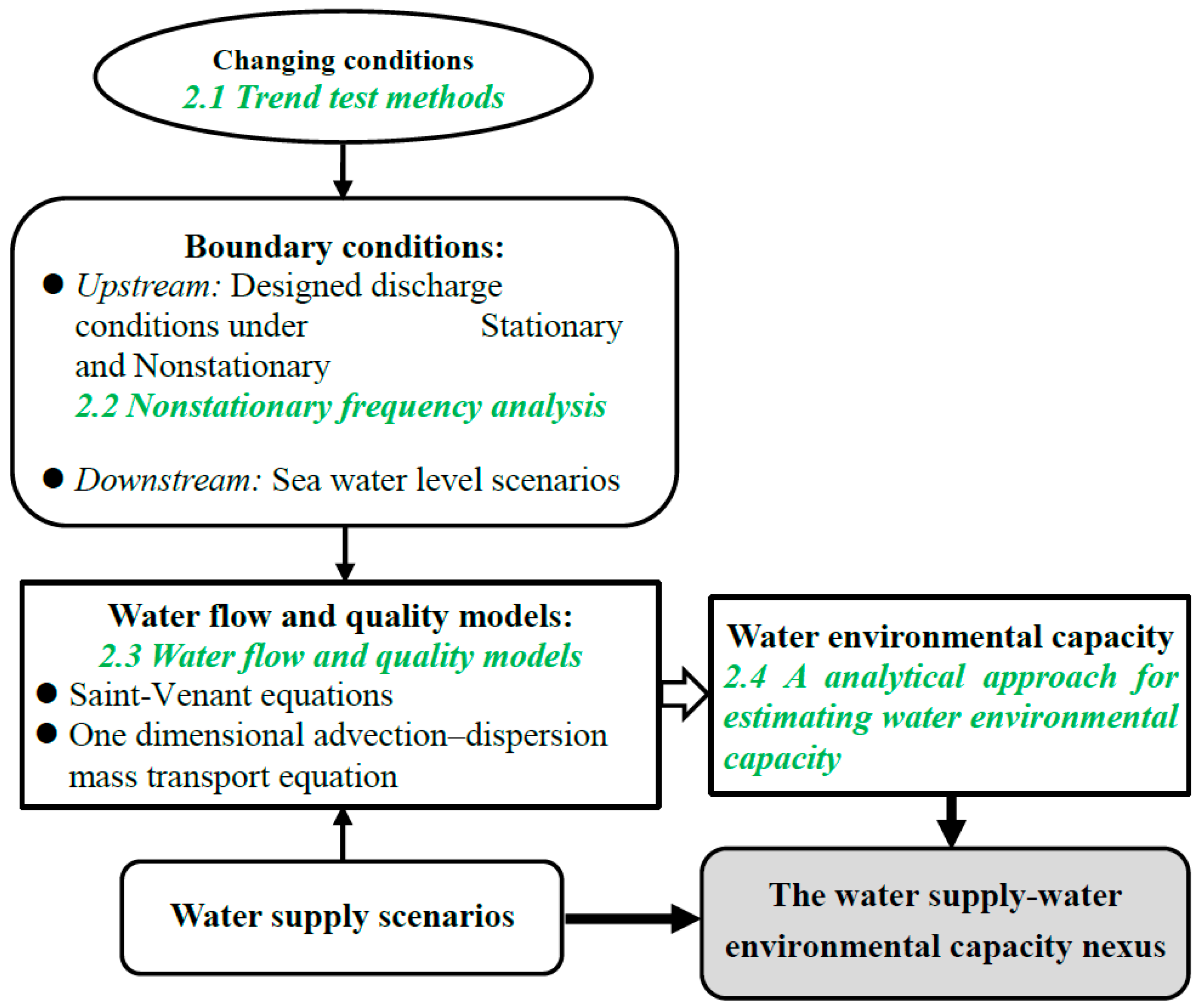
In order to construct the water supply-water environmental nexus, the water supply scenario should be set and its corresponding water environmental capacity needs to be determined through the simulation of water flow and quality. The Saint–Venant equations simulate the water flow, while the one-dimensional advection–dispersion mass transport equation in the saltwater intrusion area can simulate the water quality. The reliability of the water supply and the water environmental capacity are determined by the design water flow discharge conditions. That is, the designed water flow discharge into the saltwater intrusion area from the equivalent reliability for nonstationary frequency analysis is taken as the upstream boundary condition for the water flow and quality models. The water environmental capacity estimation can be derived from one-dimensional advection–dispersion mass transport equation and the Saint–Venant equations. The sea water level scenarios are set for the downstream boundary conditions in the models. Therefore, the computational flow chart of the water supply-water environmental capacity nexus can be as shown in Figure 1.
2.1. Nonstationary and Trend Test Methods
Defining Q as the annual minimum daily flow, the stationarity of the time series data Q can then be tested by the Kwiatkowski–Phillips–Schmidt–Shin (KPSS) test method [47]. The time series Qt is assumed to be the sum of a deterministic trend βt, random walk γt, and stationary error εt at time t in the following linear regression model [48].
and
where the μt is independent and identically distributed N(0, σu2). The initial value γ0 is treated as a fixed value and it serves as an intercept in the linear regression model. The null hypothesis for the stationarity around a deterministic trend is σu2 = 0, while the alternative hypothesis is σu2 > 0. In another case, the statistic for the level-stationary model adopts the null hypothesis as βt = 0. Kwiatkowski et al. [47] provide critical values of a certain significance level (α). The stationarity test of low flow in our study will be implemented using the function “kpsstest” in the MATLAB environment.
Qt = βt + γt + εt
γt = γt−1 + μt
The trend of the annual minimum daily flow time series will be tested using the Mann–Kendall (M–K) method and the Pettitt change point analysis will be employed to determine the change point [49,50,51]. The M–K test is a rank-based nonparametric trend detection method that is commonly used to assess the significance of monotonic trends in hydrological data time series [40,52,53,54]. The null hypothesis for no-trend in the M–K test is that the low flow time series are randomly ordered. On the contrary, the alternative hypothesis states that the series has an increasing or a decreasing monotonic trend at a certain significance level (α). If the series has a significant trend, then the significant change point will be statistically detected through Pettitt change point analysis, which is based on the first-order change point of the series. The details regarding the Pettitt change point analysis can be found in the study by Pettitt [51].
Only nonstationary low flow time series are modelled by the nonstationary frequency analysis method. For nonstationary low flow time series with significant trends (passing the M–K test), time is chosen as a covariate in the location parameters of the frequency distribution function [46,55,56]. Pearson type III is the distribution function that is recommended by the Ministry of Water Resources of China for hydrologic frequency analysis in China [57]. The nonstationary Pearson type III will be used for the frequency analysis of low flow series with nonstationary or significant trends. Nonstationary probability models always estimate the trend of location parameters under the assumption that the scale and shape parameters are fixed (e.g., [52,58,59,60]). The primary reason is that modelling the temporal changes in scale and shape parameters reliably require long-term observations that are often not available for practical applications. [35]. Therefore, the probability distribution function of the nonstationary Pearson type III is given by
where a(t), δ, and ξ are the location, scale, and shape parameters, respectively. The location parameter a(t) follows a regression model of the year, like a(t) = a0 + a1exp[a2 (t − a3)], to guarantee a positive location parameter [61,62]. The minimum Akaike information criterion (AIC) method is applied in order to estimate the parameters (i.e., a0, a1, a2, a3, δ, and ξ) of the nonstationary Pearson type III models in this study [63].
2.2. Nonstationary Frequency Analysis for the Designed Discharge Condition
The application of hydrological frequency analysis for the designed discharge condition is often framed as a risk (p0) of a hydrologic event that is below the design value X0 for water supply or environmental protection projects. If no lower value than X0 occurs during the design life of n years, then the reliability is defined as (1 − p0)n, under the assumption of independence and stationarity [64]. However, from the nonstationary perspective [7,65], the reliability (S) with which the probability of flow exceeds design quantile X0 before or at life year n under the circumstances of time-varying exceedance probabilities pt is:
If the reliability (S), as determined by Equation (1), can also be calculated through a surrogate dataset under the stationary condition, then the probability (p′ is called equivalent reliability) and its quantile value will be obtained, as follows:
where Φ−1(•) is the inverse distribution function of pt under the nonstationary condition and it is determined by Equation (3). Θ is the parameters [a0, a1, a2, a3, δ, and ξ].
2.3. Water Flow and Quality Models in a Saltwater Intrusion Area
A saltwater intrusion area is always a river delta or a plain river network area with a very complex water system. The water flow in these areas is always simulated based on Saint–Venant equations describing the mathematical translation of the laws of conservation of mass and momentum. The equations can be formulated, as shown in Equations (7) and (8) [52,66,67,68,69]:
where A is the wetted cross-sectional area (m2); Q is the flow (m3·s−1); x is the distance (m); t is the time (s); q is the lateral inflow (m3·s−1·m−1); α is the momentum correction coefficient; g is the gravitational acceleration (m ·s−2); H is the water surface elevation above datum (m); R = A/P is the hydraulic radius (m); P is the wetted perimeter (m); is the Chezy coefficient; and, n is Manning’s roughness coefficient. Because there is no analytical solution for the Saint–Venant equations, a numerical Preissmann implicit finite difference scheme is utilized [70].
A one-dimensional advection–dispersion mass transport equation is employed in order to simulate water quality. As the equation takes into account the effect of advection, dispersion, dilution, constituent reactions, interactions, flow sources, and sinks [71], for any constituent concentration C, the mass transportation phenomena can be described, as follows [72,73,74]:
where A is the cross-sectional area (m2); u is the cross-sectional averaged flow velocity (m·s−1); C is the pollutant concentration (kg·m−3); Ex is the diffusion coefficient (m2·s−1); and, Sc is the source/sink term that represents the phenomena of decay, growth, erosion, and deposition occurring in the river for non-conservative constituents (kg·m2·s−1). Sc is often converted to –KAC, where K is the comprehensive decay coefficient. An implicit implementation of the upwind difference scheme, as developed by Courant et al. [75], is used to approximate the advection term (the second term in Equation (9)). The third term (diffusion) in the equation, which represents the flux of pollutants out of the water, is approximated through the central difference scheme.
2.4. An Analytical Approach for Estimating Water Environmental Capacity in a Saltwater Intrusion River Network
The water environmental capacity estimation (W) can be derived from the water quality equation (Equation (9)) and the hydrodynamic equations (Equations (7) and (8)) as the following expression [76]:
Q0l is computed based on the Saint–Venant equation (Equations (7) and (8)) model in the saltwater intrusion area at the lth river; C0l is obtained from the monitored results in flow water quality (Equation (9)); Csl is the water quality concentration that meets the specified water environment function, and Vl is a river segment volume, which is equal to AlLl (L is the river length); LN is the total number of sub-rivers; and, ql, Al are the same as in Equations (7) and (9), respectively.
3. Study Area and Dataset
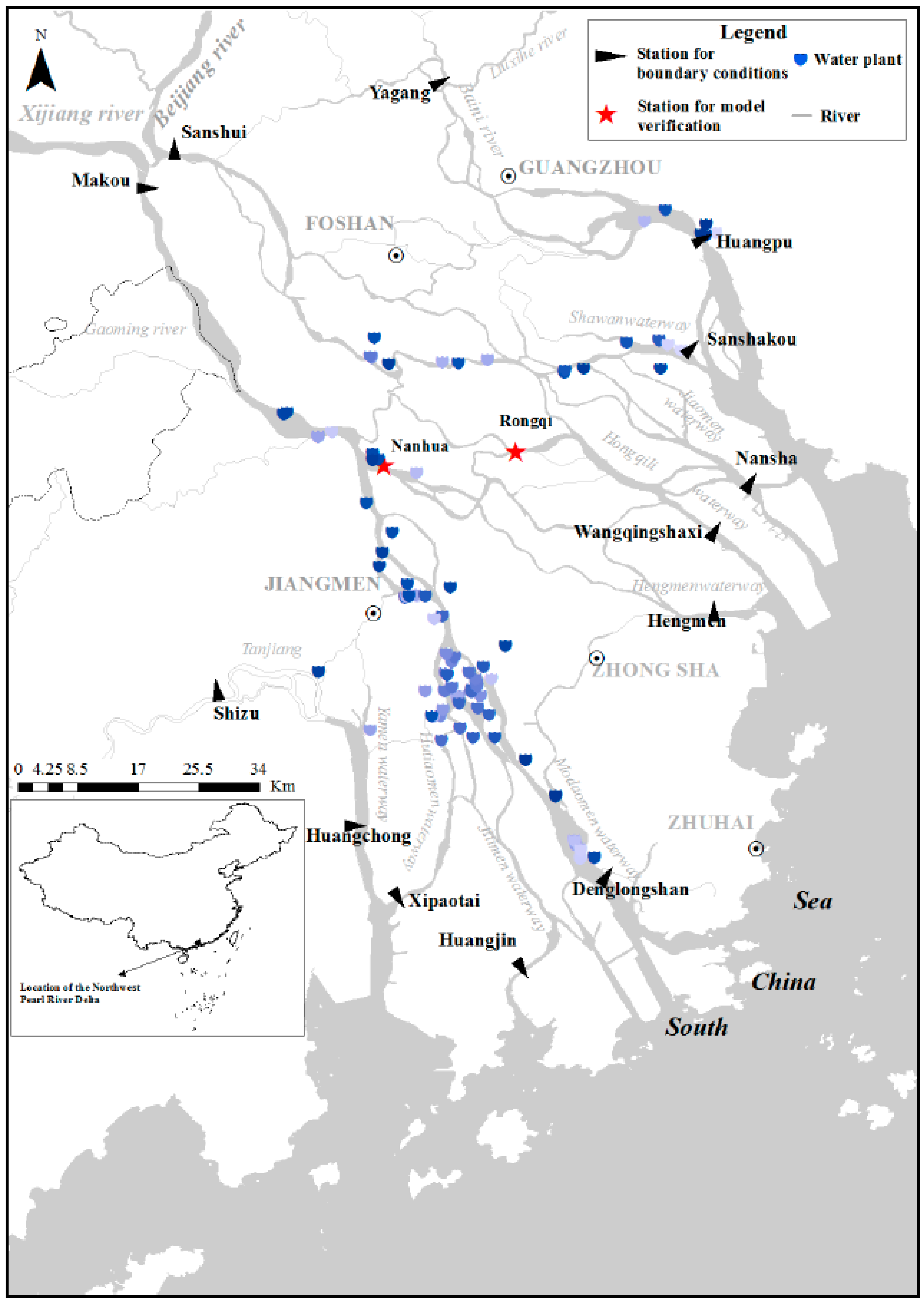
The Northwest Pearl River Delta, which is located in Guangdong Province in South China (see Figure 2), drains 18,851 square kilometres, and it is characterised by a humid climate with annual precipitations ranging from 1184 to 2679 mm (from 1959 to 2000). There are five main administrative cities, namely Guangzhou, Foshan, Jiangmen, Zhongshan, and Zhuhai, in the Guangdong province. Water is supplied through 94 waterworks intakes that are distributed as shown in Figure 1. The river networks in the Northwest Pearl River Delta are divided into 154 river units, 93 junction units, and 781 sections. 15 external units have been taken as boundary conditions, which represent the upstream discharge hydrographs (Beijiang River and Xijiang River) and the downstream water levels. The discharge data for Makou and Sanshui as the upstream boundary conditions are for the period 1959–2000. The other external unit data as boundary conditions are the water levels. As more polluted water is discharged into the rivers with increasing water consumption, the water supply-water environmental nexus has become more important for local water resource operations, especially in the dry season, when low freshwater flow in the upstream area and saltwater intrusion in the downstream area occurs.
4. Results and Discussion
4.1. Calibration and Validation of Water Flow and Quality Models in Saltwater Intrusion Area
The calibration and validation of water flow and quality models in the Northwest Pearl River Delta have been concretely described in a previous study [52]. According to intensive data collection in December of 1991, the Nash–Sutcliffe Efficiency coefficients (NSE) of the water levels were 0.89–0.95 at the observed five gauging stations. The NSE of the water level at the Nanhua and Rongqi stations were 0.983 and 0.981, while the NSE of the water discharges at the same stations were 0.849 and 0.636 in the validation process. The results of the validation confirm the goodness of fit between the observed and simulated values from the Saint–Venant equations. The integrated chemical parameter, chemical oxygen demand (COD), is considered to be an important indicator of variable water quality in our study [77]. The comprehensive decay coefficient K was assigned a value of 0.2 day−1, according to the results that were obtained from previous studies in the same area [78,79]. There was also agreement between the observed data and the model results from Equation (9) for the COD [52].
4.2. Designed Discharge Conditions for the Upstream Boundary Conditions under Climate Changes
4.2.1. Nonstationary and Trend Test for the Annual Minimum Seven-day Average Flow in the Makou and Sanshui Gauge Stations
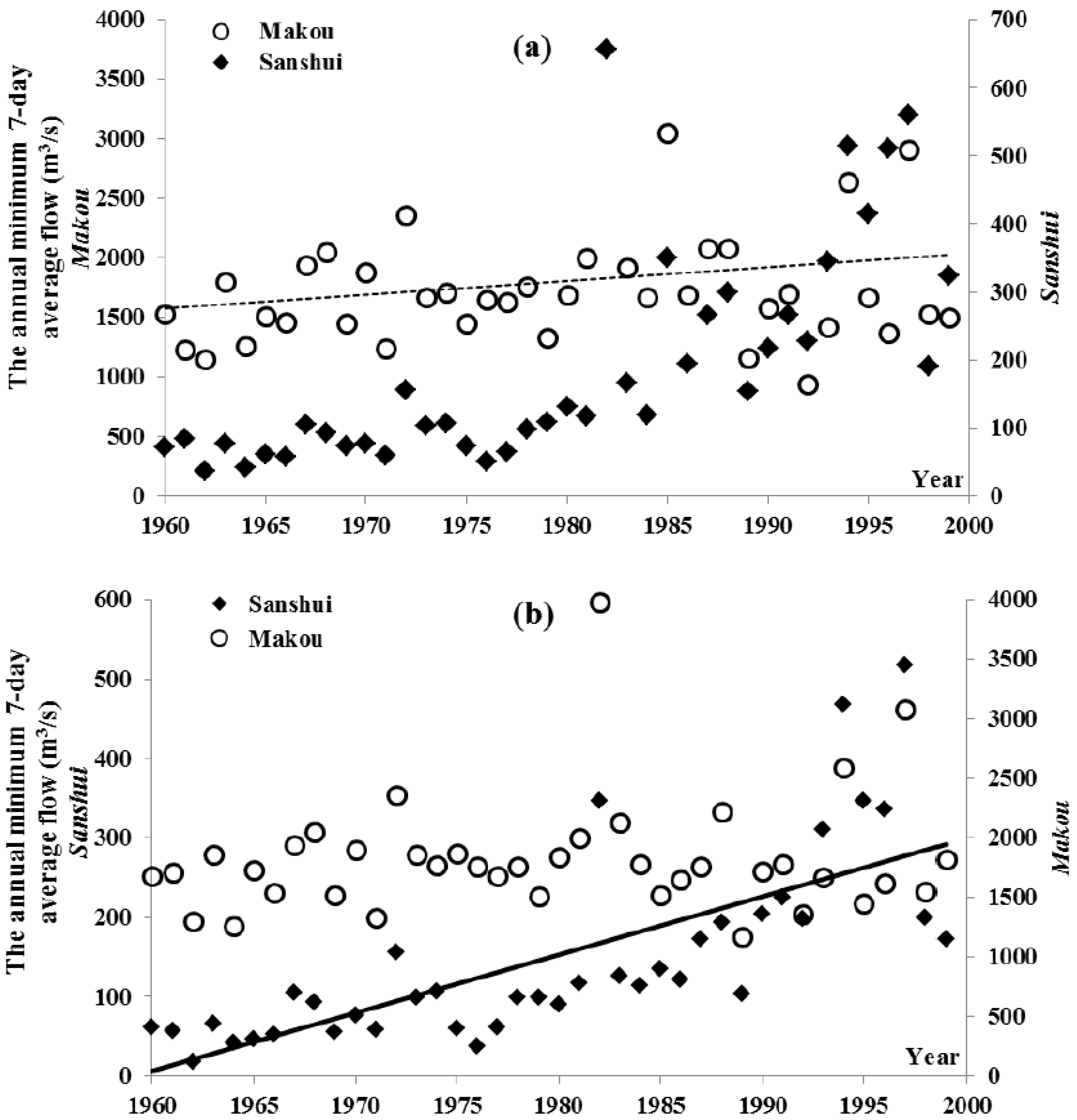
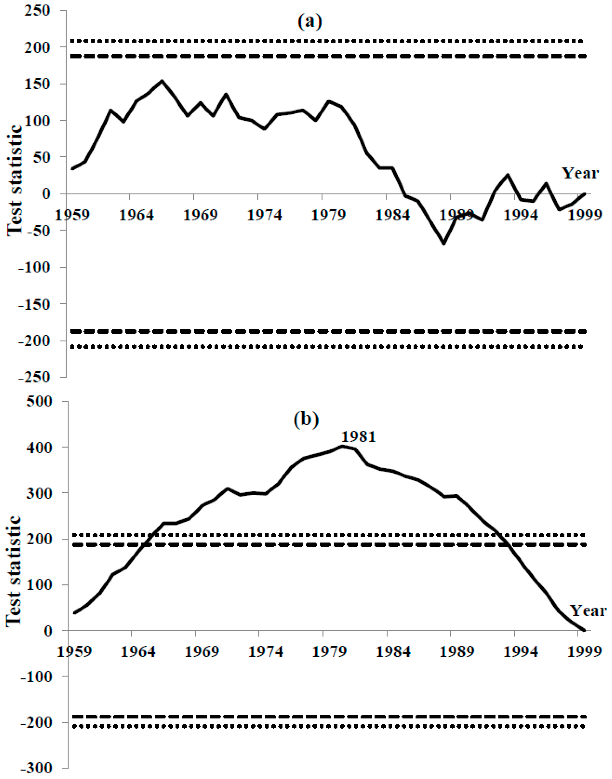
In order to assure the discharge data collected at the same time at both Makou and Sanshui gauge stations, the annual minimum seven-day average flow is chosen from one station (e.g., Makou in Figure 3a and Sanshui in Figure 3b), while the average flow during the same period will be picked up in the other station (Sanshui in Figure 3a and Makou in Figure 3b) based on the typical low-flow method. Even though the annual minimum seven-day average flow at the Makou gauging station is significantly scattered, as shown in Figure 3a, the fitted trend line does show an overall increasing trend. The stationarity test results show that only the annual minimum seven-day average flow time series in Sanshui is considered to be nonstationary at a 5% significance level. The trends of the annual minimum seven-day average flow time series are tested using the M–K test method, and the test results are displayed in Figure 4. The series in Sanshui show a significantly positive trend, and they also identify 1981 as a change point with a significance level of 5% (Figure 4b). Therefore, the 7Q10 from Sanshui (as shown in Figure 4b) should be determined through nonstationary frequency analysis, while the stationary frequency analysis is fit to the time series, as presented in the report of the ASCE that is shown in Figure 4a.
4.2.2. Q10 at Sanshui Gauge Station under Nonstationary Frequency Analysis
The regression equation for the time-varying location parameter a(t) in Equation (3) is . δ and ξ are 19.9998 and 19.9987, respectively. As a sample size of 30 years (n = 30) is commonly adopted for hydrologic frequency analysis [80], the values of the 7Q10 can be determined, as shown in Table 1, for periods 1959–1988 (for the beginning of the data series), 1979–1999 (for the last data series in the historical record), 1992–2021 (for the current data period), and 1999–2028 (for the future) through Equation (5) if p′ = 0.1. A typical low flow event over seven days was selected from the observed flow series in Sanshui based on the minimum difference between the designed 7Q10 and the observed low flow event. The low flow in Makou that happened during the same period was chosen and then converted to designed flow by multiplying the ratio of the designed 7Q10 and the observed low flow in Sanshui. In order to determine the differences between the nonstationary and stationary results, the designed low flow after 1981 was determined through stationary frequency analysis where the frequency was also 10% (as shown in the last column of Table 1). There are two water inflows in the upstream boundary, and two data time series before and the after the changed point in every water inflow series, and four scenarios can be formed under the nonstationary condition. As there is another assumed stationary series, five scenarios for the upstream boundary conditions are set according to the results, as also shown in Table 1.
The results of the nonstationary frequency analyse are different from those from the stationary frequency analyse, which will impact the size of water environmental capacity and then the pollutant control activities in environmental management. The designed low flow under stationary conditions was slightly different from the results in 1992–2021, when the stationary condition was implemented, and the designed low flow under nonstationary conditions increased with time. The low flow freshwater in Sanshui and Makou is the upstream boundary for the Northwest Pearl River Delta. Its increase will be beneficial for the water supply and water environmental capacity.
4.3. The Water Supply-Water Environmental Capacity Nexus under Changing Boundary Conditions
4.3.1. The Nexuses under Changing Upstream Boundary Conditions
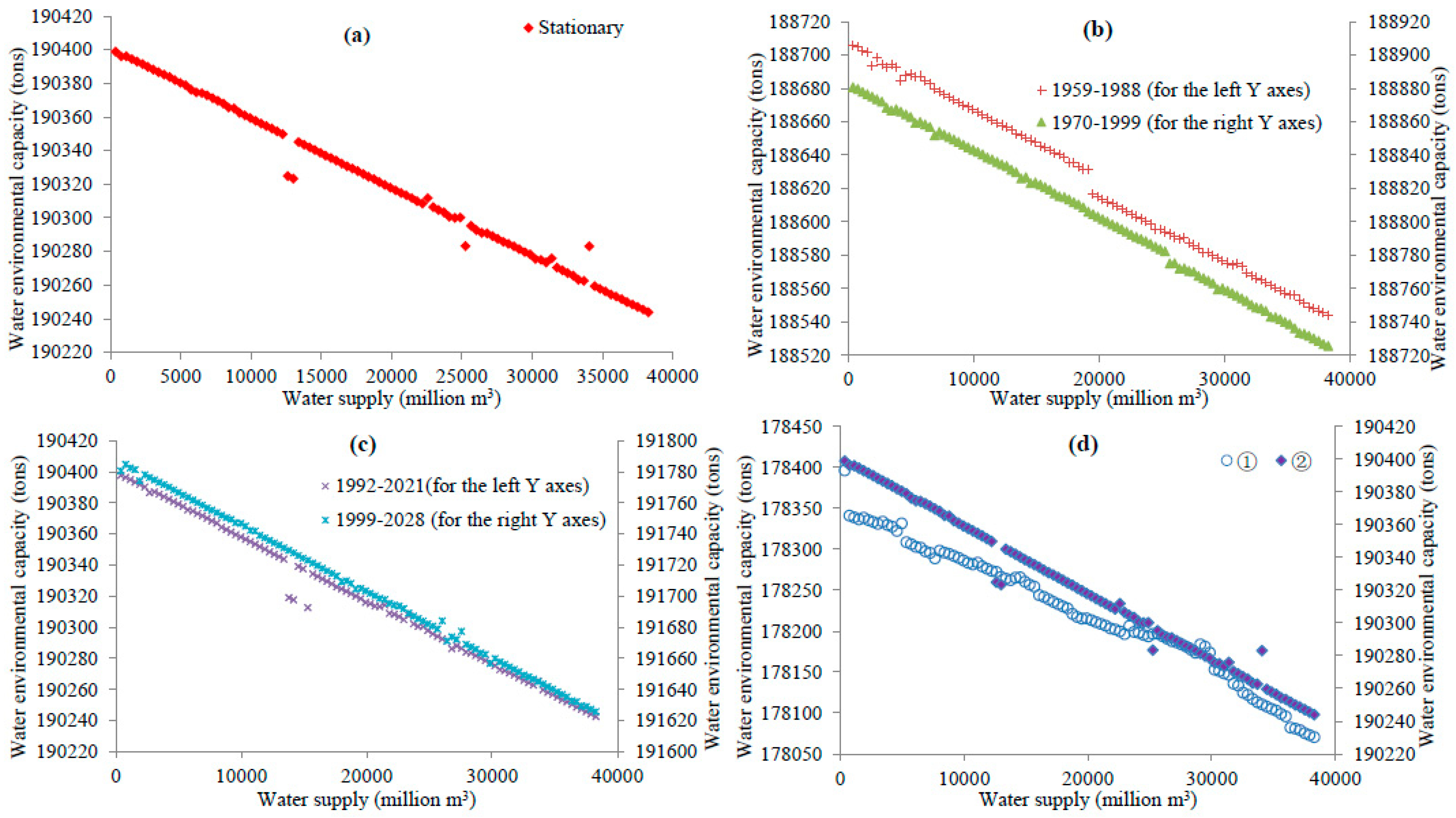
The total capacity of water supply from 94 water plants is 3710 million m3 per year. In order to present the impact of the amount of water supply on water environmental capacity, the amount of supplied water varied from 0.1 to 10 times the total capacity of the water plants, that is, between 371 and 37,100 million m3 per year, and the amount of water was converted into the discharge flow rate with units in m3 per second (from 11.76 to 1176 m3/s). Five scenarios for upstream boundary conditions are provided to the water flow and quality models to estimate the water environmental capacity (as shown in Figure 5a), while the water levels downstream are fixed according to the designed boundary conditions. Figure 5a) illustrates the relationship between water supply in million cubic meters and water environmental capacity in tons. While the amount of supplied water increases by 0.1 times the total water plant capacity, the water environmental capacity only decreases slightly under the five scenarios. On the other hand, the water environmental capacities under the five scenarios vary with the upstream boundary water flow conditions. The designed water flow increases, and the water environmental capacities increase. As the designed water flow under the future scenario is the maximum value among the scenarios, its environmental water capacity is also the largest (shown in Figure 5a). There are two factors that impact the water supply-water environmental capacity nexus in our study area. The first one is the designed freshwater flow. The water can only be supplied when the direction of water flow is downstream. Thus, the amount of water supply is determined by the five designed water flows under upstream boundary conditions. The other factor is the water levels under downstream boundary conditions. The South China Sea water level and the law of tides dominate the water levels at the downstream boundary water gates (as shown in Figure 2). As the water environmental capacity is expressed by COD instead of chlorosity in our study, saltwater can also dilute COD and increase the amount of water environmental capacity. The nexuses of the water supply-water environmental capacity seem to be declined straight lines, as shown in Figure 5a–c, on the assumption of fixed water levels in the downstream boundary conditions. However, if the saltwater cannot dilute COD and assume the amount of water environmental capacity to be zero when the water flow runs upward driven by saltwater. The water environmental capacity is shown in Figure 5d, which is zoomed in under the stationary condition. The nexus of water supply-water environmental capacity is changed into a declined curved line.
4.3.2. The Nexuses under Changing Downstream Boundary Conditions
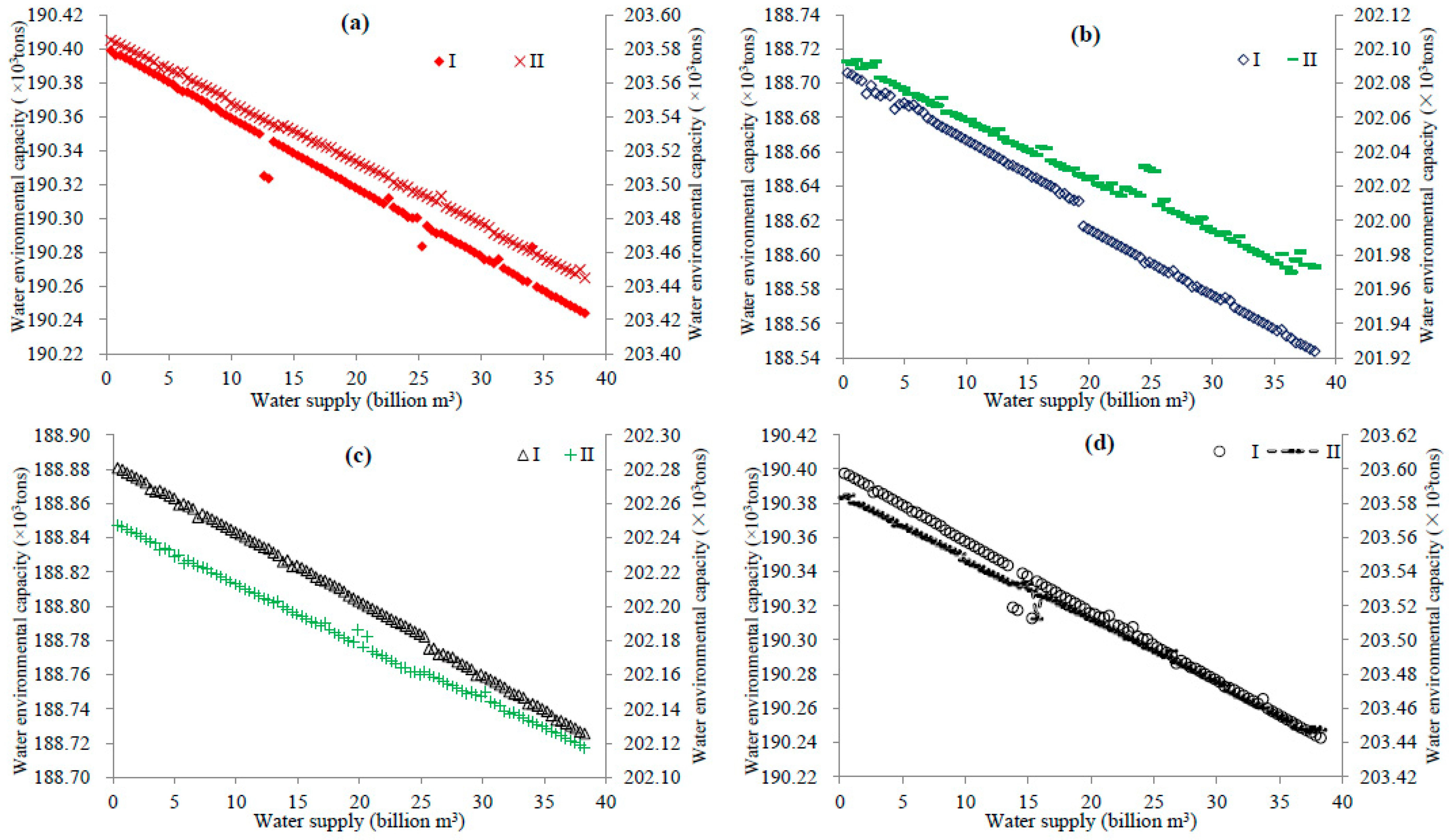
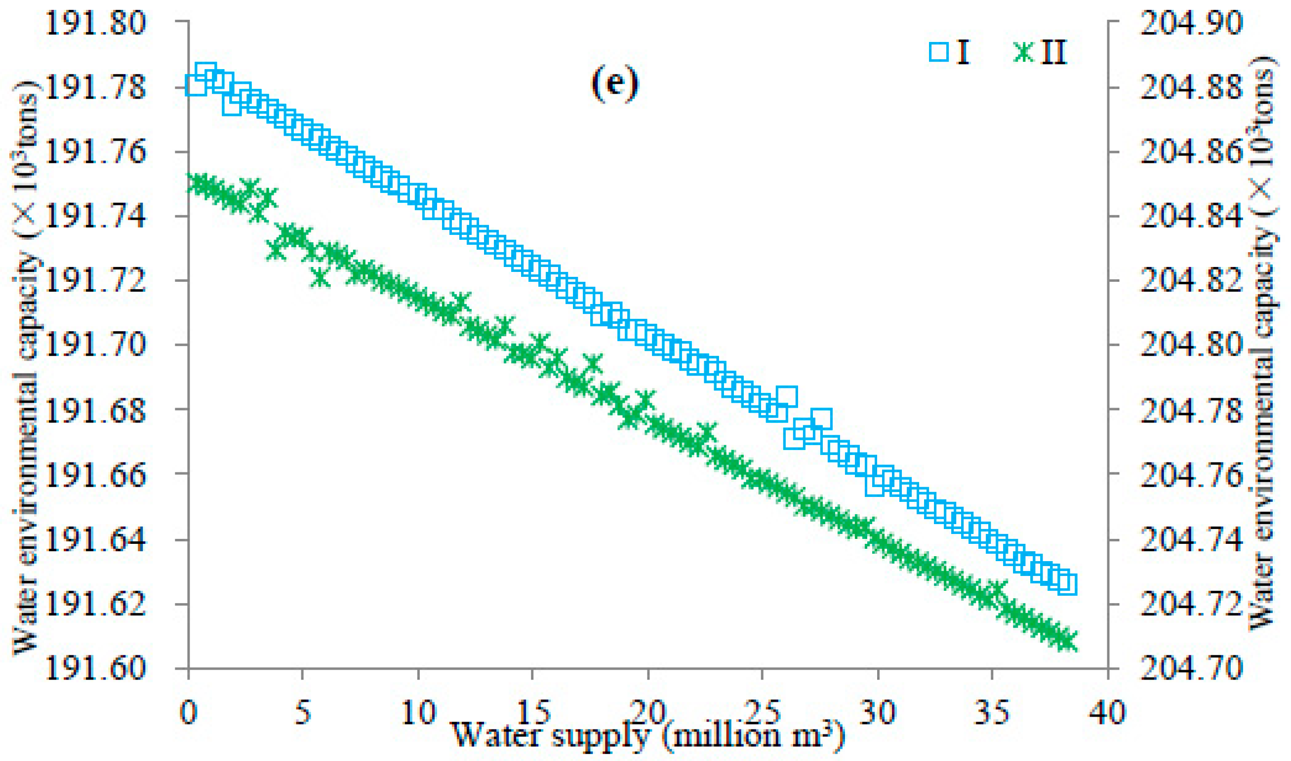
In order to investigate the impacts of water level conditions at downstream boundaries on the nexuses of water supply-water environmental capacity, the water levels were assumed to increase by 0.5 m. The nexuses under rising water levels at the downstream boundaries are shown in Figure 6. Figure 6a–e shows the nexuses under the conditions of rising water levels at the downstream boundaries and different upstream boundary conditions, as set out in Table 1. Figure 6a–e indicates that water environmental capacities increase with rising water level, as shown in the right sides of y-axis values. The water environmental capacity of an increasing 0.5 m water level is bigger than the original downstream water level conditions. As the freshwater in the upstream boundary became nonstationary (increasing or decreasing), the amount of water supply fluctuated. However, the water environmental capacity was impacted by the designed water flow at the upstream boundary, and by the water levels at the downstream boundary. As there is an increasing trend of designed water flow under nonstationary conditions, and the water levels at the downstream boundary are rising from the sea level, the water environmental capacity will increase. The water supply-water environment nexus in a saltwater intrusion area is impacted by both the upstream boundary water inflow and downstream boundary water level conditions. The fluctuated water inflow and the rising sea level are the two primary factors for the nexus of water supply and the pollutant control sectors.
5. Conclusions
In this paper, we developed a framework to quantify the water supply-water environment nexus in a saltwater intrusion area under nonstationary conditions. We examined this nexus by imposing nonstationary designed water flow at the upstream boundary and rising water levels at the downstream boundary, respectively. Saint–Venant equations and the one-dimensional advection–dispersion mass transport equation were employed to determine the water environmental capacity under changing boundary conditions, and these two types of equations are impacted by water supply. The models for simulating water flow and water quality in the saltwater intrusion area were solved by using the numerical Preissmann implicit finite difference scheme and the central difference scheme. Equivalent probability determined the designed water flow under nonstationary conditions.
Five scenarios under nonstationary upstream water flow conditions and two scenarios based on the assumption of rising water level at the downstream boundary were examined. The capacity of the water supply was determined by the designed freshwater flow, while the water environmental capacity was impacted by both the designed water flow at the upstream boundary and the water levels at the downstream boundary. As there was an increasing trend in the designed flow, the water environmental capacity should also increase. As the salt intrusion water can dilute COD, which increases the water environmental capacity, the nexuses of water supply-water environmental capacity seem to be constant lines for saltwater intrusion areas. Our research results can also help in water quality protection in the river-reservoir system, where the impacts of reservoir operation on its tail area are analogous to tide intrusions.
Author Contributions
Conceptualization, D.L. and Y.Q.; Methodology, D.L.; Software, D.L. and Y.Q.; Validation, D.L., Y.Z., Y.S. and J.Z.; Formal Analysis, D.L.; Investigation, D.L. and Y.Q.; Resources, D.L. and Y.Q.; Data Curation, D.L., Y.Z.; Writing-Original Draft Preparation, D.L.; Writing-Review & Editing, D.L.; Visualization, D.L. and Y.Z.; Supervision, D.L.; Project Administration, D.L.; Funding Acquisition, D.L.
Funding
This research was funded by the National Natural Science Foundation of China (Nos. 91647106, 51579183, 51879194 and 51525902), 111 Project (No. B18037).
Conflicts of Interest
We declare that we do not have any commercial or associative interest that represents a conflict of interest in connection with the work submitted.
References
- Vörösmarty, C.J. Global Water Resources: Vulnerability from Climate Change and Population Growth. Science 2000, 289, 284–288. [Google Scholar] [CrossRef]
- Ercin, A.E.; Hoekstra, A.Y. Water footprint scenarios for 2050: A global analysis. Environ. Int. 2014, 64, 71–82. [Google Scholar] [CrossRef] [PubMed]
- Xie, Z.; Xu, L.; Liu, L.; Duan, X.; Xu, X. Analysis of boundary adjustments and land use policy change—A case study of Tianjin Palaeocoast and Wetland National Natural Reserve, China. Ocean & Coastal Management 2012, 56, 56–63. [Google Scholar]
- Arrow, K.; Bolin, B.; Costanza, R.; Dasgupta, P.; Folke, C.; Holling, C.S.; Jansson, B.-O.; Levin, S.; Maler, K.-G.; Perrings, C.; et al. Economic Growth, Carrying Capacity, and the Environment. Ecol. Econ. 1995, 15, 89–90. [Google Scholar] [CrossRef]
- Keller, A.A.; Cavallaro, L. Assessing the US clean water Act 303(d) listing process for determining impairment of a water body. J. Environ. Manag. 2008, 86, 699–711. [Google Scholar] [CrossRef] [PubMed]
- Li, Y.; Qiu, R.; Yang, Z.; Li, C.; Yu, J. Parameter determination to calculate water environmental capacity in Zhangweinan Canal Sub-basin in China. J. Environn. Sci. 2010, 22, 904–907. [Google Scholar] [CrossRef]
- Milly, P.C.D.; Betancourt, J.; Falkenmark, M.; Hirsch, R.M.; Kundzewicz, Z.W.; Lettenmaier, D.P.; Stouffer, R.J. Stationarity is dead: whither water management? Science 2008, 319, 573–574. [Google Scholar] [CrossRef]
- WEF (World Economic Forum). Water Security: The Water–Food–Energy–Climate Nexus; Island Press: Washington, DC, USA, 2012. [Google Scholar]
- Cai, X.; Wallington, K.; Shafiee-Jood, M.; Marston, L. Understanding and managing the food-energy-water nexus – opportunities for water resources research. Adv Water Resour. 2018, 111, 259–273. [Google Scholar] [CrossRef]
- Biggs, E.M.; Bruce, E.; Boruff, B.; Duncan, J.M.; Horsley, J.; Pauli, N.; McNeill, K.; Neef, A.; Van Ogtrop, F.; Curnow, J.; et al. Sustainable development and the water–energy–food nexus: A perspective on livelihoods. Environ. Sci. Policy 2015, 54, 389–397. [Google Scholar] [CrossRef]
- Maass, A.; Hufschmidt, M.M.; Dorfman, R.; Thomas, H.A., Jr.; Marglin, S.A.; Fair, G.M. Design of Water-Resource Systems: New Techniques for Relating Economic Objectives, Engineering Analysis, and Governmental Planning; Harvard University Press: Cambridge, UK; Macmillan: London, UK, 1962. [Google Scholar]
- Global Water Partnership. Towards Water Security: A Framework for Action. Report Prepared for presentation at the Second World Water Forum, The Hague, The Netherlands, 17–22 March 2000; Global Water Partnership: Stockholm, Sweden, 2000; p. 120. [Google Scholar]
- Hanlon, P.; Madel, R.; Olson-Sawyer, K.; Rabin, K.; Rose, J. Food, Water and Energy: Know the Nexus; GRACE Communications Foundation: New York, NY, USA, 2013. [Google Scholar]
- Hoff, H. Understanding the Nexus. Background Paper for the Bonn 2011 Nexus Conference: The Water, Energy and Food Security Nexus Solution for the Green Economy; Stockholm Environment Institute: Stockholm, Sweden, 2011. [Google Scholar]
- Ringler, C.; Bhaduri, A.; Lawford, R. The nexus across water, energy, land and food (WELF): Potential for improved resource use efficiency? Curr. Opin. Environ. Sustain. 2013, 5, 617–624. [Google Scholar] [CrossRef]
- Rasul, G. Food, water, and energy security in South Asia: A nexus perspective from the Hindu Kush Himalayan region. Environ. Sci. Policy 2014, 39, 35–48. [Google Scholar] [CrossRef]
- Keairns, D.L.; Darton, R.C.; Irabien, A. The Energy-Water-Food Nexus. Annu. Rev. Chem. Biomol. Eng. 2016, 7, 239–262. [Google Scholar] [CrossRef] [PubMed]
- Saladini, F.; Betti, G.; Ferragina, E.; Bouraoui, F.; Cupertino, S.; Canitano, G.; Gigliotti, M.; Autino, A.; Pulselli, F.; Riccaboni, A.; et al. Linking the water-energy-food nexus and sustainable development indicators for the Mediterranean region. Ecol. Indic. 2018, 91, 689–697. [Google Scholar] [CrossRef]
- Cherchi, C.; Badruzzaman, M.; Oppenheimer, J.; Bros, C.M.; Jacangelo, J.G. Energy and water quality management systems for water utility’s operations: A review. J. Environ. Manag. 2015, 153, 108–120. [Google Scholar] [CrossRef] [PubMed]
- Feng, M.; Liu, P.; Li, Z.; Zhang, J.; Liu, D.; Xiong, L. Modeling the nexus across water supply, power generation and environment systems using the system dynamics approach: Hehuang Region, China. J. Hydrol. 2016, 543, 344–359. [Google Scholar] [CrossRef]
- Shahzad, M.W.; Burhan, M.; Ang, L.; Ng, K.C. Energy-water-environment nexus underpinning future desalination sustainability. Desalination 2017, 413, 52–64. [Google Scholar] [CrossRef]
- Stigson, P. The Resource Nexus: Linkages Between Resource Systems. Ref. Modu. Earth Syst. Environ. Sci. 2013, 13. [Google Scholar] [CrossRef]
- Al-Ansari, T.; Korre, A.; Nie, Z.; Shah, N. Development of a life cycle assessment tool for the assessment of food production systems within the energy, water and food nexus. Sustain. Prod. Consum. 2015, 2, 52–66. [Google Scholar] [CrossRef]
- Feng, K.; Hubacek, K.; Siu, Y.L.; Li, X. The energy and water nexus in Chinese electricity production: A hybrid life cycle analysis. Renew. Sustain. Energy Rev. 2014, 39, 342–355. [Google Scholar] [CrossRef]
- Chang, Y.; Huang, R.; Ries, R.J.; Masanet, E. Life-cycle comparison of greenhouse gas emissions and water consumption for coal and shale gas fired power generation in China. Energy 2015, 86, 335–343. [Google Scholar] [CrossRef]
- Walker, R.V.; Beck, M.B. Understanding the metabolism of urban-rural ecosystems. Urban Ecosyst. 2012, 15, 809–848. [Google Scholar] [CrossRef]
- Nanduri, V.; Saavedra-Antolínez, V. A competitive Marko decision process model for the energy-water-climate change nexus. Appl Energ. 2013, 111, 186–198. [Google Scholar] [CrossRef]
- Karaca, F.; Raven, P.G.; Machell, J.; Camci, F. A comparative analysis framework for assessing the sustainability of a combined water and energy infrastructure. Technol. Forecast. Soc. Chang. 2015, 90, 456–468. [Google Scholar] [CrossRef]
- Endo, A.; Burnett, K.; Orencio, P.M.; Kumazawa, T.; Wada, C.A.; Ishii, A.; Tsurita, I.; Taniguchi, M. Methods of the Water-Energy-Food Nexus. Water 2015, 7, 5806–5830. [Google Scholar] [CrossRef]
- IPCC (Intergovernmental Panel on Climate Change). Climate Change 2007: The Physical Science Basis, Working Group 1, IPCC Fourth Assessment Report; Cambridge University Press: Cambridge, UK, 2007. [Google Scholar] [CrossRef]
- Katz, R.W.; Parlange, M.B.; Naveau, P. Statistics of extremes in hydrology. Adv. Water Resour. 2002, 25, 1287–1304. [Google Scholar] [CrossRef]
- Cooley, D. Return Periods and Return Levels Under Climate Change; Springer: Dordrecht, The Netherlands, 2013; Volume 65, pp. 97–114. [Google Scholar]
- Parey, S.; Hoang, T.T.H.; Dacunha-Castelle, D. Different ways to compute temperature return levels in the climate change context. Environmetrics 2010, 21, 698–718. [Google Scholar] [CrossRef]
- Rootzén, H.; Katz, R. Design Life Level: Quantifying risk in a changing climate. Water Resour. Res. 2013, 49, 5964–5972. [Google Scholar] [CrossRef]
- Cheng, L.; AghaKouchak, A.; Gilleland, E.; Katz, R.W. Non-stationary extreme value analysis in a changing climate. Climatic Change 2014, 127, 353–369. [Google Scholar] [CrossRef]
- Obeysekera, J.; Salas, J.D. Frequency of Recurrent Extremes under Nonstationarity. J. Hydrol. Eng. 2016, 21, 4016005. [Google Scholar] [CrossRef]
- Hu, Y.; Liang, Z.; Singh, V.P.; Zhang, X.; Wang, J.; Li, B.; Wang, H. Concept of Equivalent Reliability for Estimating the Design Flood under Non-stationary Conditions. Water Resour. Manag. 2018, 32, 997–1011. [Google Scholar] [CrossRef]
- Xu, Z.X.; Lu, S.Q. Research on hydrodynamic and water quality model for tidal river networks. J. Hydrodyn. Ser. B 2003, 15, 64–70. [Google Scholar]
- Hu, J.; Zhang, J.; Han, L. Water Supply System Dispatching Considering the Influence of Salt Water Intrusion in Coastal City; American Society of Civil Engineers (ASCE): Washington, DC, USA, 2011; pp. 4649–4657. [Google Scholar]
- Liu, D.; Chen, X.; Lian, Y.; Lou, Z. Impacts of climate change and human activities on surface runoff in the Dongjiang River basin of China. Hydrol. Process. 2010, 24, 1487–1495. [Google Scholar] [CrossRef]
- Karamouz, M.; Kerachian, R.; Mahmoodian, M. Waste-Load Allocation Model for Seasonal River Water Quality Management: Application of Sequential Dynamic Genetic Algorithms. Sci. Iran. 2003, 12, 117–130. [Google Scholar]
- United States Environmental Protection Agency (USEPA). Terms of Environment: Glossary, Abbreviations, and Acronyms; EPA Office of Communications, Education, and Public Affairs: Galveston, TX, USA, 1997.
- Ames, D.P. Estimating 7Q10 Confidence Limits from Data: A Bootstrap Approach. J. Water Resour. Plann. Manag. 2006, 132, 204–208. [Google Scholar] [CrossRef]
- Ministry of Water Resources the People’s Republic of China (MWR). Code of Practice for Computation on Permissible Pollution Bearing Capacity of Water Bodies SL 348-2006; Ministry of Water Resources the People’s Republic of China (MWR): Beijing, China, 2016. (In Chinese)
- American Society of Civil Engineering (ASCE). Task Committee on Low-Flow Evaluation, Methods, and Needs of the Committee on SurfaceWater Hydrology of the Hydraulics Division. Charact. Low Flows Proc. Pap. 1980, 106, 717–731. [Google Scholar]
- Rossel, V.; De La Fuente, A. Assessing the link between environmental flow, hydropeaking operation and water quality of reservoirs. Ecolo. Eng. 2015, 85, 26–38. [Google Scholar] [CrossRef]
- Kwiatkowski, D.; Phillips, P.C.; Schmidt, P. Testing the Null Hypothesis of Stationarity Against the Alternative of a Unit Root: How Sure Are We That Economic Time Series Have a Unit Root? J. Econ. 1992, 54, 159–178. [Google Scholar] [CrossRef]
- Gao, M.; Mo, D.; Wu, X. Nonstationary modeling of extreme precipitation in China. Atmos. Res. 2016, 182, 1–9. [Google Scholar] [CrossRef]
- Kendall, M.G. Rank Correlation Measures; Charles Griffin: London, UK, 1975. [Google Scholar]
- Mann, H.B. Nonparametric tests against trend. Econometrica 1945, 13, 245–259. [Google Scholar] [CrossRef]
- Pettitt, A.N. A non-parametric approach to the change point problem. Appl. Stat. 1979, 28, 125–135. [Google Scholar] [CrossRef]
- Liu, D.; Guo, S.; Lian, Y.; Xiong, L.; Chen, X. Climate-informed low-flow frequency analysis using nonstationary modelling. Hydrol. Process. 2014, 29, 2112–2124. [Google Scholar] [CrossRef]
- Rashid, M.M.; Beecham, S.; Chowdhury, R.K. Assessment of trends in point rainfall using Continuous Wavelet Transforms. Adv. Water Resour. 2015, 82, 1–15. [Google Scholar] [CrossRef]
- Foulon, É.; Rousseau, A.N.; Gagnon, P. Development of a methodology to assess future trends in low flows at the watershed scale using solely climate data. J. Hydrol. 2018, 557, 774–790. [Google Scholar] [CrossRef]
- AghaKouchak, A.; Eaterling, D.; Hsu, K.; Schubert, S.; Sorooshian, S. Extremes in a Changing Climate; Springer: New York, NY, USA, 2013. [Google Scholar]
- Um, M.-J.; Kim, Y.; Markus, M.; Wuebbles, D.J. Modeling nonstationary extreme value distributions with nonlinear functions: An application using multiple precipitation projections for U.S. cities. J. Hydrol. 2017, 552, 396–406. [Google Scholar] [CrossRef]
- Ministry of Water Resources the People’s Republic of China (MWR). Regulation for Calculating Design Flood of Water Resources and Hydropower Projects (SL44-2006); China Water Power Press: Beijing, China. (In Chinese)
- Leclerc, M.; Ouarda, T.B. Non-stationary regional flood frequency analysis at ungauged sites. J. Hydrol. 2007, 343, 254–265. [Google Scholar] [CrossRef]
- Zwiers, F.W.; Zhang, X.; Feng, Y. Anthropogenic Influence on Long Return Period Daily Temperature Extremes at Regional Scales. J. Climate 2011, 24, 881–892. [Google Scholar] [CrossRef]
- Westra, S.; Alexander, L.; Zwiers, F.W. Global Increasing Trends in Annual Maximum Daily Precipitation. J. Climate 2013, 26, 3904–3918. [Google Scholar] [CrossRef]
- Villarini, G.; Stron, A. Roles of climate and agricultural practices in discharge changes in anagricultural watershed in Iowa. Agrc. Ecosyst. Environ. 2014, 188, 204–211. [Google Scholar] [CrossRef]
- Lima, C.H.; Lall, U.; Troy, T.J.; Devineni, N. A climate informed model for nonstationary flood risk prediction: Application to Negro River at Manaus, Amazonia. J. Hydrol. 2015, 522, 594–602. [Google Scholar] [CrossRef]
- Akaike, H. A New Look at the Statistical Model Identification. IEEE T Automat Contr. 1974, 19, 716–723. [Google Scholar] [CrossRef]
- Haan, C.T. Statistical Methods in Hydrology; Iowa State University Press: Iowa, IA, USA, 2002. [Google Scholar]
- Milly, P.C.D.; Betancourt, J.; Falkenmark, M.; Hirsch, R.M.; Kundzewicz, Z.W.; Lettenmaier, D.P.; Stouffer, R.J.; Dettinger, M.D.; Krysanova, V. On critiques of “Stationarity is dead: Whither water management?”. Water Resour. Res. 2015, 51, 7785–7789. [Google Scholar] [CrossRef]
- De Saint-Venant. Théorie du Mouvement non Permanent des Eaux, Avec Application aux Crues des Rivières et à L’introduction des Marées dans Leur Lit; Gauthier-Villars: Paris, France, 1871. (In French) [Google Scholar]
- Cunge, J.A.; Holly, F.M.; Verwey, A. Practical Aspects of Computational River Hydraulics; Pitman Advanced Publishing Program: Boston, UK, 1980. [Google Scholar]
- Litrico, X.; Fromion, V.; Baume, J.-P.; Arranja, C.; Rijo, M. Experimental validation of a methodology to control irrigation canals based on Saint-Venant equations. Control Eng. Pract. 2005, 13, 1425–1437. [Google Scholar] [CrossRef]
- Launay, M.; Le Coz, J.; Camenen, B.; Walter, C.; Angot, H.; Dramais, G.; Faure, J.-B.; Coquery, M. Calibrating pollutant dispersion in 1-D hydraulic models of river networks. J. Hydro-Environ. Res. 2015, 9, 120–132. [Google Scholar] [CrossRef]
- Preissmann, A. Propagation des intumescenes dans lescanaux et rivières. In Ler Congress de L’Assoc; Francaise de Calcul: Grenoble, France, 1960. [Google Scholar]
- Kerachian, R.; Karamouz, M. A stochastic conflict resolution model for water quality management in reservoir–river systems. Adv. Water Resour. 2007, 30, 866–882. [Google Scholar] [CrossRef]
- Lopes, L.F.G.; Carmo, J.S.D.; Cortes, R.M.V.; Oliveira, D. Hydrodynamics and water quality modelling in a regulated river segment: application on the instream flow definition. Ecol. Model. 2004, 173, 197–218. [Google Scholar] [CrossRef]
- Liu, W.-C.; Kuo, J.-T.; Kuo, A.Y. Modelling hydrodynamics and water quality in the separation waterway of the Yulin offshore industrial park, Taiwan. Environ. Model. Softw. 2005, 20, 309–328. [Google Scholar] [CrossRef]
- Kilic, S.G.; Aral, M.M. A fugacity based continuous and dynamic fate and transport model for river networks and its application to Altamaha River. Sci. Total Environ. 2009, 407, 3855–3866. [Google Scholar] [CrossRef] [PubMed]
- Courant, R.; Isaacson, E.; Rees, M. On the solution of nonlinear hyperbolic differential equations by finite differences. Commun. Pur. Appl. Math. 1952, 5, 243–255. [Google Scholar] [CrossRef]
- Yao, Y.-J.; Yin, H.-L.; Li, S. The computation approach for water environmental capacity in tidal river network. J. Hydrodyn. Ser. B 2006, 18, 273–277. [Google Scholar] [CrossRef]
- Zhou, N.; Westrich, B.; Jiang, S.; Wang, Y. A coupling simulation based on a hydrodynamics and water quality model of the Pearl River Delta, China. J. Hydrol. 2011, 396, 267–276. [Google Scholar] [CrossRef]
- South China Institute of Environmental Science (SCIES). Report on Surface Water Environmental Capacity for Guangdong Province, China; South China Institute of Environmental Science (SCIES): Guangzhou, China, 2005. (In Chinese) [Google Scholar]
- Guangdong Provincial Department of Water Resources (GDWR). Water Resources Protection Planning of Guangdong Province Report; Guangdong Provincial Department of Water Resources (GDWR): Guangzhou, China, 2002. [Google Scholar]
- Li, H.; Sun, J.; Zhang, H.; Zhang, J.; Jung, K.; Kim, J.; Xuan, Y.; Wang, X.; Li, F. What Large Sample Size Is Sufficient for Hydrologic Frequency Analysis?—A Rational Argument for a 30-Year Hydrologic Sample Size in Water Resources Management. Water 2018, 10, 430. [Google Scholar] [CrossRef]
Figure 1.
Schematic computational flow chart of water supply-water environmental capacity nexus: all “ ![Water 11 00346 i001]() ” are the inputs for water flow and quality models. “
” are the inputs for water flow and quality models. “ ![Water 11 00346 i002]() ” is the inputs for water environmental capacity while “
” is the inputs for water environmental capacity while “ ![Water 11 00346 i003]() ” indicates the input for the nexus.
” indicates the input for the nexus.
 ” are the inputs for water flow and quality models. “
  ” is the inputs for water environmental capacity while “
  ” indicates the input for the nexus.
Figure 1.
Schematic computational flow chart of water supply-water environmental capacity nexus: all “ ![Water 11 00346 i001]() ” are the inputs for water flow and quality models. “
” are the inputs for water flow and quality models. “ ![Water 11 00346 i002]() ” is the inputs for water environmental capacity while “
” is the inputs for water environmental capacity while “ ![Water 11 00346 i003]() ” indicates the input for the nexus.
” indicates the input for the nexus.
” are the inputs for water flow and quality models. “ ” is the inputs for water environmental capacity while “ ” indicates the input for the nexus.
Figure 2.
Location of the Northwest Pearl River Delta (The shade ![Water 11 00346 i004]() of indicates the size of water plant, the deeper blue, and its bigger size).
of indicates the size of water plant, the deeper blue, and its bigger size).
 of indicates the size of water plant, the deeper blue, and its bigger size).
Figure 2.
Location of the Northwest Pearl River Delta (The shade ![Water 11 00346 i004]() of indicates the size of water plant, the deeper blue, and its bigger size).
of indicates the size of water plant, the deeper blue, and its bigger size).
of indicates the size of water plant, the deeper blue, and its bigger size).
Figure 3.
The annual minimum seven-day low flow as a function of time and the corresponding linear at (a) Makou (dashedline) and (b) Sanshui station (solid line). Their simultaneously flows at Sanshui in (a) oratMakou in (b) are also presented, respectively.
Figure 3.
The annual minimum seven-day low flow as a function of time and the corresponding linear at (a) Makou (dashedline) and (b) Sanshui station (solid line). Their simultaneously flows at Sanshui in (a) oratMakou in (b) are also presented, respectively.

Figure 4.
The annual minimum low flow change point at (a) Makou and (b) Sanshui stations. Horizontal lines represent the significance levels of 5% (dotted) and 10% (dashed).
Figure 4.
The annual minimum low flow change point at (a) Makou and (b) Sanshui stations. Horizontal lines represent the significance levels of 5% (dotted) and 10% (dashed).

Figure 5.
Supply-water environmental capacity nexus under the changing upstream boundary conditions: (a–c) the salt intrusion water can increase the water environmental capacity under the different boundary conditions; (d) the Comparison between salt intrusion water increase (indicated by “①” for the left Y axes) and cannot increase (indicated by “②” for the right Y axes) the water environmental capacity under the stationary boundary conditions.

Figure 6.
Supply-water environmental capacity nexus responded to the downstream boundary scenarios: “I” is the result of the figure 5with original downstream boundary condition corresponding to the left Y axes while “II” represents the water levels increased by 0.5m corresponding to the right Y axes. (a) Stationary, (b) 1959–1988, (c) 1970–1999, (d) 1992–2021, and (e) 1999–2028represent the upstream water inflow boundary condition.


Table 1.
7Q10 for Sanshui station and its corresponding low flow at Makou according to the typical low flow method (m3/s).
Table 1.
7Q10 for Sanshui station and its corresponding low flow at Makou according to the typical low flow method (m3/s).
| Station | Nostationary | Stationary * | |||
|---|---|---|---|---|---|
| 1959–1988 | 1970–1999 | 1992–2021 | 1999–2028 | ||
| Sanshui | 32.24 | 34.81 | 87.40 | 192.29 | 87.43 |
| Makou | 1080.29 | 1166.45 | 1792.13 | 2214.41 | 1792.66 |
* Stationary condition is satisfied after 1982 in Sanshui flow series.
© 2019 by the authors. Licensee MDPI, Basel, Switzerland. This article is an open access article distributed under the terms and conditions of the Creative Commons Attribution (CC BY) license (http://creativecommons.org/licenses/by/4.0/).
Share and Cite
MDPI and ACS Style
Liu, D.; Zeng, Y.; Qin, Y.; Shen, Y.; Zhang, J. Water Supply-Water Environmental Capacity Nexus in a Saltwater Intrusion Area under Nonstationary Conditions. Water 2019, 11, 346. https://doi.org/10.3390/w11020346
AMA Style
Liu D, Zeng Y, Qin Y, Shen Y, Zhang J. Water Supply-Water Environmental Capacity Nexus in a Saltwater Intrusion Area under Nonstationary Conditions. Water. 2019; 11(2):346. https://doi.org/10.3390/w11020346
Chicago/Turabian StyleLiu, Dedi, Yujie Zeng, Yue Qin, Youjiang Shen, and Jiayu Zhang. 2019. "Water Supply-Water Environmental Capacity Nexus in a Saltwater Intrusion Area under Nonstationary Conditions" Water 11, no. 2: 346. https://doi.org/10.3390/w11020346
Note that from the first issue of 2016, this journal uses article numbers instead of page numbers. See further details here.