Decision Support System Tool to Reduce the Energy Consumption of Water Abstraction from Aquifers for Irrigation


1
Renewable Energy Research Institute, Section of Solar and Energy Efficiency, C/ de la Investigación 1, 02071 Albacete, Spain
2
Department of Plant Production and Agricultural Technology, School of Advanced Agricultural Engineering, University of Castilla-La Mancha. Campus Universitario, s/n, 02071 Albacete, Spain
3
Regional Centre of Water Research, Castilla-La Mancha University, Campus Universitario s/n, 02071 Albacete, Spain
4
Institute for Regional Development, University of Castilla-La Mancha. Campus Universitario, s/n, 02071 Albacete, Spain
*
Author to whom correspondence should be addressed.
Water 2019, 11(2), 323; https://doi.org/10.3390/w11020323
Submission received: 20 December 2018
/
Revised: 2 February 2019
/
Accepted: 12 February 2019
/
Published: 14 February 2019
(This article belongs to the Special Issue Modelling and Management of Irrigation System)
Abstract
:In pressurized irrigation networks that use underground water resources, submersible pumps are one of the highest energy consumers. The objective of this paper was to develop a decision support system, implemented in MATLAB®, to reduce the energy consumption of the water abstraction process, from an aquifer to a reservoir in existing wells, by installing a frequency speed drive. An economic module with the aim to assess the economic profitability of the investment cost of the variable speed drive was also developed. This tool was used in three wells that were located in the Eastern Mancha Aquifer. Several scenarios and irrigation seasons were analyzed while considering the interannual and annual variation in ground water depth. In the three analyzed irrigation societies (named A, B, and C), energy savings were achieved using a variable speed frequency when compared with fixed speed. Considering the analyzed cases, when the dynamic water table level is higher, energy savings ranged from 4.4% and 24.4%, using a variable speed ratio of 0.9 and 0.82. The energy savings based on the variable speed frequency increased when the dynamic water table level was lower, with the average energy savings close to 23%, 22% and 6.8% for irrigation societies A, B, and C, respectively. The results also show that the investment costs of the variable speed drive in two of the three irrigation societies studied were highly profitable, with a payback that ranged from 4.5 to 10 years.
1. Introduction
In most countries of the world, the use of underground water resources has a relevant importance, mainly in arid and semiarid climates. Approximately one-third of the landmass in the world is irrigated by groundwater. This water source is widely used in agriculture, representing 45% of the irrigated land that uses groundwater in the United States of America, 58% in Iran, and 67% in Algeria [1]. Groundwater is important in regions of Spain, such as in the Castilla–La Mancha region, where that approximate source of water represents more than 65% of water use in irrigation and urban networks [2]. In these areas, it is necessary to improve the energy that is consumed, which guarantees the economic sustainability of irrigation societies, where energy costs have increased during the last years.
Regarding groundwater resources, one relevant point to highlight is water discharge and recharge phenomena. In this regard, several sources of recharge mainly come from precipitation and surface-water bodies, such as streams, ponds, or lakes. One of the most common recharge sources is the irrigation water, mainly when the amount of water applied to crops exceed the crop water requirements. Regarding the discharge, flow into streams or groundwater pumped from wells is also common. Water recharged to groundwater for years has a high variability, because it depends on the amount of precipitation or the local geology of each irrigable area.
Some tools have been developed to improve water and energy use in irrigation networks, considering the energy efficiency of the pumping systems or the irrigation scheduling management at the plot scale [3,4]. Most of those studies did not consider the energy efficiency from wells, which, in most of cases, they do not work with adequate efficiency.
In pressurized networks that use those resources, the energy consumed is a factor to be considered, which represents a high participation of the total management, operation, and maintenance costs [5]. In those areas, water is extracted from the aquifer using submersible pumps with high installed power depending on the water table level. The influence of the use of underground water resources can be highlighted when comparing the average values of the energy cost per unit of irrigation delivery in water users’ associations (WUAs) [6]. For instance, in the Castilla-La Mancha Region (Spain), the energy costs per cubic meter delivery ranged from 0.022 € m−3 to 0.026 € m−3 in WUAs with sprinkler irrigation systems and with drip irrigation systems, respectively. These costs did not include the costs of water abstraction from wells. If these costs were considered, the energy costs calculated for sprinkler and drip irrigation systems would increase, reaching values close to 0.061 € m−3 and 0.071 € m−3, respectively. These costs are very similar in both irrigation systems. It was explained because in all irrigation societies analyzed, the average head supply by the pumping systems were very similar between sprinkler irrigation systems (58 m) and drip irrigation systems (53 m), besides energy efficiency for each pump of the pumping stations.
Most of the studies carried out in pressurized irrigation networks are focused on the study of energy efficiency in pumping stations, which pump water from a reservoir. In some cases, these studies are based on determining the irrigation sectoring methodologies to improve energy management [7,8,9,10,11]. In other cases, a comparison of several types of regulation systems in pumping stations is evaluated, considering the efficiency of the pumping system for each combination of flow discharge and pressure head [9,12,13].
In some energy audits carried out in the Castilla–La Mancha region [14], it can be highlighted that the submersible pumps are one of the highest energy consumers in these types of associations, reaching up to 70% of the energy cost.
For that reason, it is necessary to analyze the performance and energy efficiency in wells. Some studies are focused on determining the optimal well discharge [15,16,17,18]. Other researchers [19] tried to optimize the characteristics and efficiency curves in the pumping wells that delivered to a pivot irrigation system. In that study, a methodology was carried out to determine the minimum total water application cost (investment plus operation costs), while optimizing the diameters of the pumping pipes, distribution pipes, and lateral pipes.
In wells, the most typical management approach is to work with a fixed speed frequency during the whole irrigation season; however, an analysis that can evaluate the energy savings of using a frequency speed drive to manage the water abstraction from wells has not been found.
The aim of this paper was to develop a decision support system tool, named DSSW (Decision Support System for Water abstraction), to determine the effect of installing frequency speed drives in wells on the energy savings and cost recovery in managing the underground water abstraction process. Several scenarios were analyzed in three wells with different characteristics that are located in the Eastern Mancha Aquifer (Spain). This work complements previous studies focused on the improvement of energy efficiency at irrigable areas, such as MOPECO [20] or GREDRIP model [4], used to determine irrigation schedules and to estimate the relationship between irrigated crop yield and net water applied. In this regard, the use of DSSW does not depend on the water applied at each irrigation network, because it establishes the energy savings and cost recovery independently of the total irrigation applied at each irrigable area. The variation in the dynamic water table level in different irrigation seasons was evaluated. For each scenario, the operating point was computed with several variable speed frequencies to determine the minimum energy consumed per cubic meter of water delivery, compared with the fixed speed frequency. An economic analysis of installing this type of device was also performed to evaluate the economic profitability of this action.
2. Methodology
2.1. Description of the DSSW Tool
The DSSW tool was developed in MATLAB® (MathWorks Inc., MA, USA) to simulate the performance of wells using fixed and variable speed pumping, as well as the energy consumption for each type of management approach. An energy analysis of different indicators and the main energy variables was accurately calculated. By applying the DSSW tool, it was possible to determine the viability of installing a frequency speed drive to minimize the energy consumption per cubic meter of water extracted from the aquifer. With this aim, the followings steps were taken:
- Characterization of the analyzed wells by considering the actual water table levels during the irrigation season, along with the hydraulic characteristics of the pumping pipe diameter, material, length, location of the reservoir (distance from the well and difference in elevation), and the type and model of the pump (characteristic and efficiency curves).
- Calculation of the system curve for the different analyzed scenarios throughout the irrigation season.
- Calculation of the operating point of the pump and energy consumption, which determines the ratio of energy consumed per cubic meter (kWh m−3).
- Simulation of the well performance using a frequency speed drive with several variable speed ratios to calculate the most efficient pump speed.
- Energy analysis to account for the energy savings by using a frequency speed drive.
- Economic analysis.
The implemented tool has four modules: (1) Pumping system module, which simulates the variable speed pump performance; (2) hydraulic module, which determines the system curve accurately by considering the hydrogeologic parameter of the well and the characteristics of the pipes; (3) energy module, which determines the operating point of the system under steady state conditions and calculates the energy rates to determine the energy efficiency for each rotation speed of the pump; and (4) economic analysis module, which determines the economic profitability of the different scenarios studied in module 3.
2.1.1. Pumping System Module
The pumping system module considered the characteristics and efficiency curves of the analyzed pump, H-Q and η-Q, as indicated in Equations (1) and (2), respectively. These curves were obtained from the theoretical data provided by the pump manufacturer.
where H is the pumping head in m; Q is the flow discharge in l min−1; η is the pump efficiency at fixed speed in percentage; and a, b, c, e, and f are coefficients of the adjusted model, which define the shape of the curves.
To define the performance of the pump at different rotation speeds, the characteristics and efficiency curves for each speed were obtained using the affinity laws. Therefore, for a variable speed drive, the characteristic curves can be defined as follows:
where Hvs is the pumping head at a variable speed in m; ηvs is the pump efficiency at fixed speed in %; and α is the ratio between the speed of the variable speed drive and the maximum speed as a fixed speed drive. In addition, the efficiency of the variable speed drive for different frequencies have been taken into account according to [9].
2.1.2. Hydraulic Model
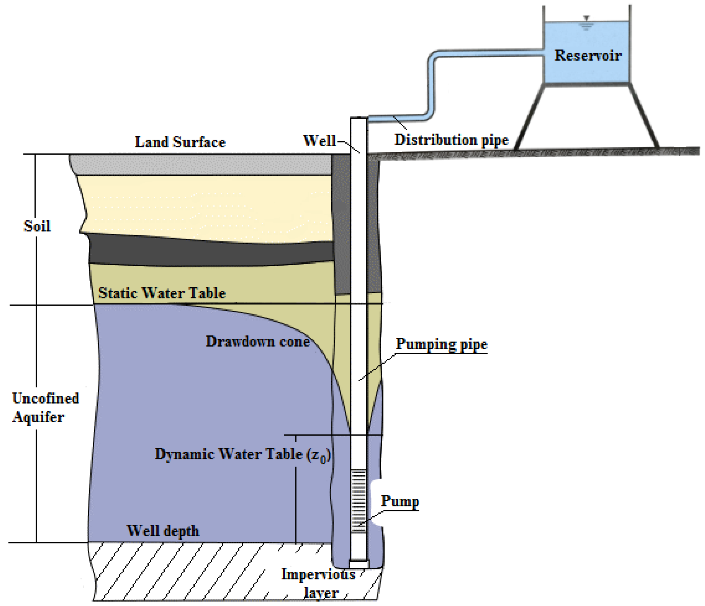
This module allowed for the system curve to be determined. In this study, the system was composed of a pump, the pumping pipe from the submersible pump to the head of the well and the distribution pipe from the head of the well to the discharge (Figure 1). Accordingly, the system curve was computed to introduce the data related to the dynamic water table level (Zo), the reference level of water discharged (Zf) at the top of the reservoir, the pipe diameter (D), the pipe length (L), and the Hazen–William coefficient (C) of the pumping pipe and the distribution pipe [2].
2.1.3. Energy Module
Once the system curve and characteristic curves for the fixed pump were implemented, the operating point was computed, which can be defined as the intersection of the system curve and the pump characteristic curve [21,22]. Hence, according to the studied system curve, it was possible to determine the operating point at each variable speed. In the proposed tool, several variable speed ratios (α) were used, one while the pump was working at maximum speed (α = 1) and the rest while the pump was activated with the frequency speed drive, which ranged from a minimum α to the maximum speed, at 0.02 intervals. Those parameters can be modified in the tool by the user.
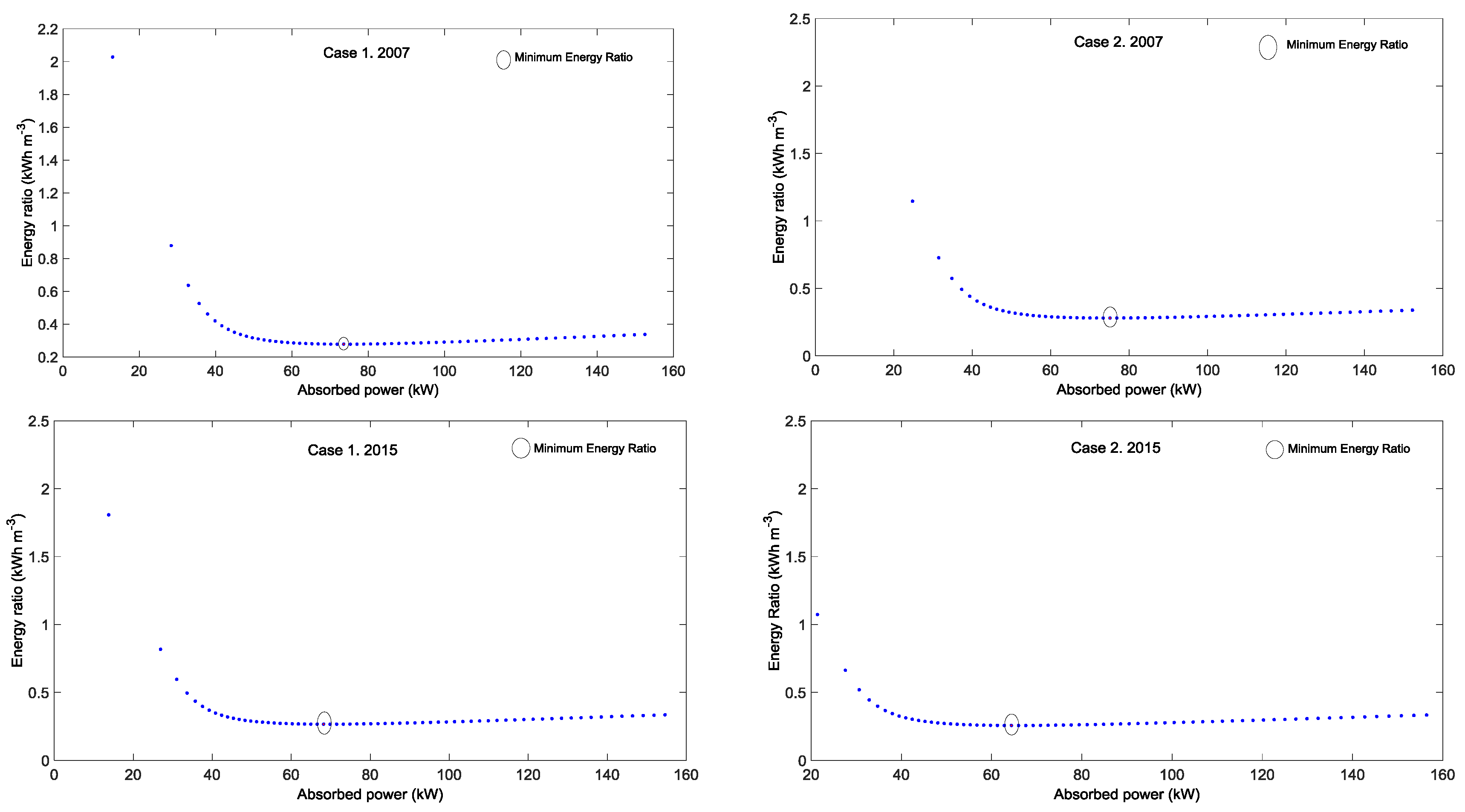
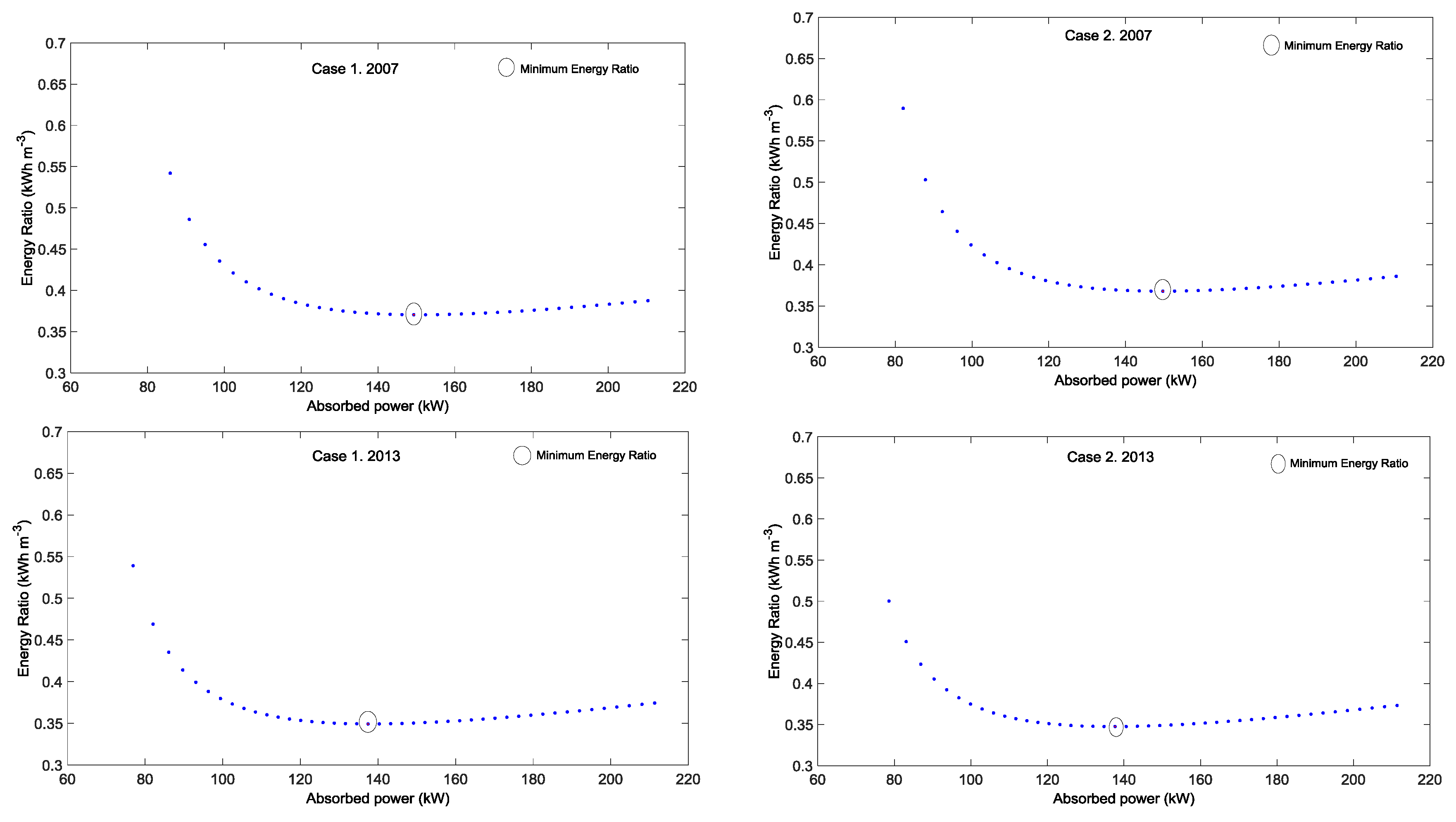
According to the previous information, at each variable speed ratio, several parameters were automatically computed, such as the pumping head (H, m), the flow discharge (Q, l min−1), efficiency (η, %), and absorbed power (Na, kW) by the pump. Moreover, at each variable speed ratio, the consumed energy was computed using the energy ratio indicator (ER, kW h m−3), which is defined as the relationship between the energy consumed per volume of water delivered. Installed power describes the nominal power of the motor (mechanical power at the motor axis) while the absorbed power is the electrical power absorbed by the motor under each demand condition (low for low frequencies of the frequency speed drive, high for maximum frequency). The absorbed power also changes for the same frequency depending on the hydraulic power (i.e., changes in the water table level). Therefore, the variable speed drive that minimizes the ER was determined, which was useful for obtaining the energy savings and comparing the use of fixed and variable speed pumps.
2.1.4. Economic Analysis Module
With the aim to determine the economic profitability of the different scenarios analyzed by comparing the use of fixed and variable speed pumps, an economic analysis module was implemented in the DSSW tool. Considering the energy savings by comparing the use of fixed and variable speed pumps, this module analyzes the economic profitability of the variable speed drive investment. Thus, Equation (5) shows the relationship between the variable speed drive and its installed power.
where Cvs is the variable speed drive cost in €; Pvs is the installed power in kW.
Equation (5) was obtained from the 13 main speed variable drive manufacturers in the Spanish market. According to these manufacturers, an annual maintenance cost of 5% of the variable speed drive cost and a lifespan of 15 years were considered in the economic analysis.
Based on Equation (5), which calculates the annual maintenance cost, lifespan, and the energy savings with variable speed pumps, this module computes the net present value (NPVvs in €), which determines the profitability of the investment, as well as the internal rate of return (IRRvs) and the payback period of the variable speed drive investment. Thus, the DSSW tool can determine the economic profitability of each study case.
2.2. Case Studies
The DSSW tool was applied to three WUAs, named A, B, and C, from the Castilla–La Mancha region, which were representative of the irrigable areas of this region. All the WUAs had similar characteristics, with the use of underground water resources as the main source of water. At each area, groundwater was pumped to a storage reservoir from which it was then pumped into the irrigation network by a pumping station. These areas were managed under a rotational schedule with on-demand management, and the command area ranged from 267 to 863 ha (Table 1). In these areas, the dynamic water table (DWT) level in the 2007 ranged from 71 (WUA B) to 105 m (WUA A). There were annual variations of the DWT, but the interannual variation of this variable was much higher.
The main characteristics of the submersible pumps and the required data for the tool at each one of the analyzed WUAs are shown in Table 2.
With the aim to compute the energy consumption by each WUA, the water volume applied in each irrigation season was recorded. The water volumes applied were similar in each irrigation season. Thus, average applied water volumes of 836,225 m3, 601,136 m3, and 170,535 m3 for WUA A, WUA B, and WUA C, respectively, were considered. Finally, the unit energy cost of the study region was 0.10 € kWh−1.
2.3. Data Acquisition
At each of the analyzed wells, the hydraulic, electrical and topographic parameters were measured during the peak period (July) of the 2007 irrigation season. This information was useful for determining the performance of each of the analyzed wells. Regarding the hydraulic data, the flow rate was measured using a portable ultrasound flow meter (2.5% accuracy) at the pump discharge pipe. In addition, the DWT level was measured with a portable electric contact meter. The electrical parameters, such as the current, voltage, power factor, and absorbed power, were obtained using an electrical network analyzer (1.5% accuracy). Regarding the topographic parameters, such as the top of the reservoir, where water was discharged, and the head of well, were measured using GNSS-RTK equipment (with an error of less than 1 cm). Thus, the operating point was measured (discharge, pressure, and efficiency) and compared with the theoretical characteristic and efficiency curves.
2.4. Water Table Level Analysis
In this study, an analysis of the influence of the water table level on the operating point at different pump rotation speeds was carried out. It was applied for several irrigation seasons, using the water table level information from the selected piezometer database.
In the whole Jucar Basin, in which the analyzed WUAs were located, there was a dense network of piezometers (www.chj.es). Monthly data from each piezometer since the early sixties were available. However, there were many gaps in the available data, and a proper selection of the most representative piezometers for each WUA was performed.
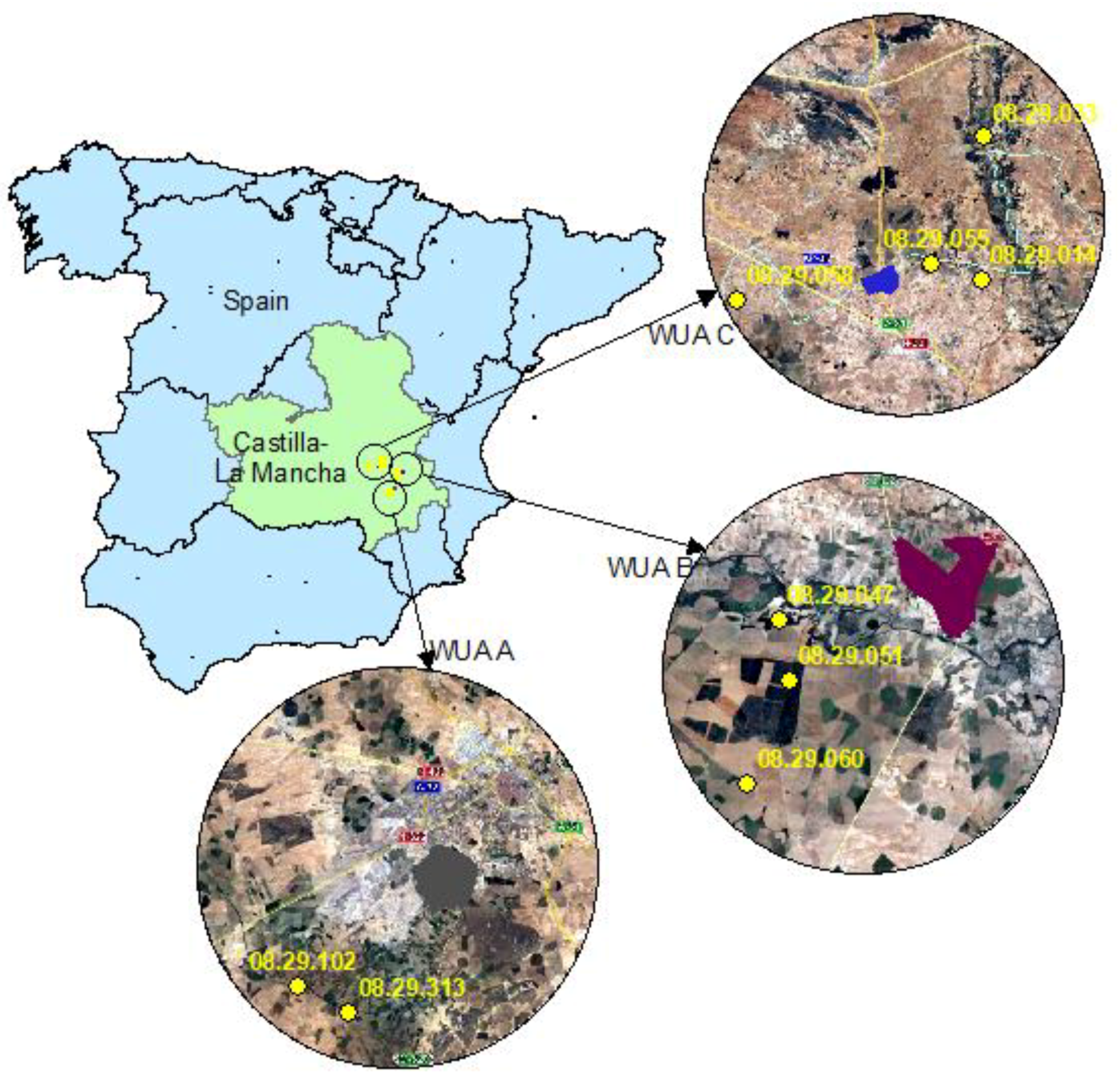
At each piezometer, the available information included monthly values of the static water table (SWL) level at each irrigation season. Table 3 shows the identification (Id) of each piezometer, as well as their UTM (Universal Transverse Mercator) coordinates and the data available period for each water users’ association. In WUA A, information about two piezometers was available (08.29.102 and 08.29.313), with monthly data of the SWT level from 2007 to 2013. In WUA B, three piezometers were available (08.29.047, 08.29.051, and 08.29.060), with SWT information from 2007 to 2013 and 2015. In WUA C, four piezometers had available information, piezometers 08.29.033 and 08.29.058 (information from 2007 to 2013), 08.29.055 (information from 2007 to 2011), and 08.29.014 (from 2008 to 2013). The location for each piezometer is shown in Figure 2.
Once the piezometer database was available for each analyzed well, it was possible to estimate the actual DWT level for each month of the analyzed irrigation seasons. To compute the DWT, we had information about the DWT measured in July 2007, in all the analyzed cases. It was measured during energy audits carried out in that irrigation season [14]. It was measured using a portable SEBA-electric contact meter. Hence, using the DWT measured data as the main reference, the percentage of annual and interannual variation was calculated with the original data of the piezometers related to SWT. The same variation for the SWT was applied to the DWT measured in 2007 to obtain DWT values for the rest of analyzed irrigation seasons.
In addition, for each irrigation season, three cases (Case 1, Case 2, and Case 3) were proposed, with the aim to define an average DWT level for each case during the corresponding irrigation season. These cases were proposed to analyze the annual DWT variation. Therefore, Case 1 represented the average DWT level for a period with high crop water requirements (from June to August), Case 2 (from March to May), and Case 3 (from September to November) represented the average DWT level for a period with low crop water requirements. Although the developed tool is capable of evaluating as many scenarios as a user can define (monthly or even daily), we decided to simplify the case studies to demonstrate the results more clearly.
3. Results and Discussion
3.1. Operating Point
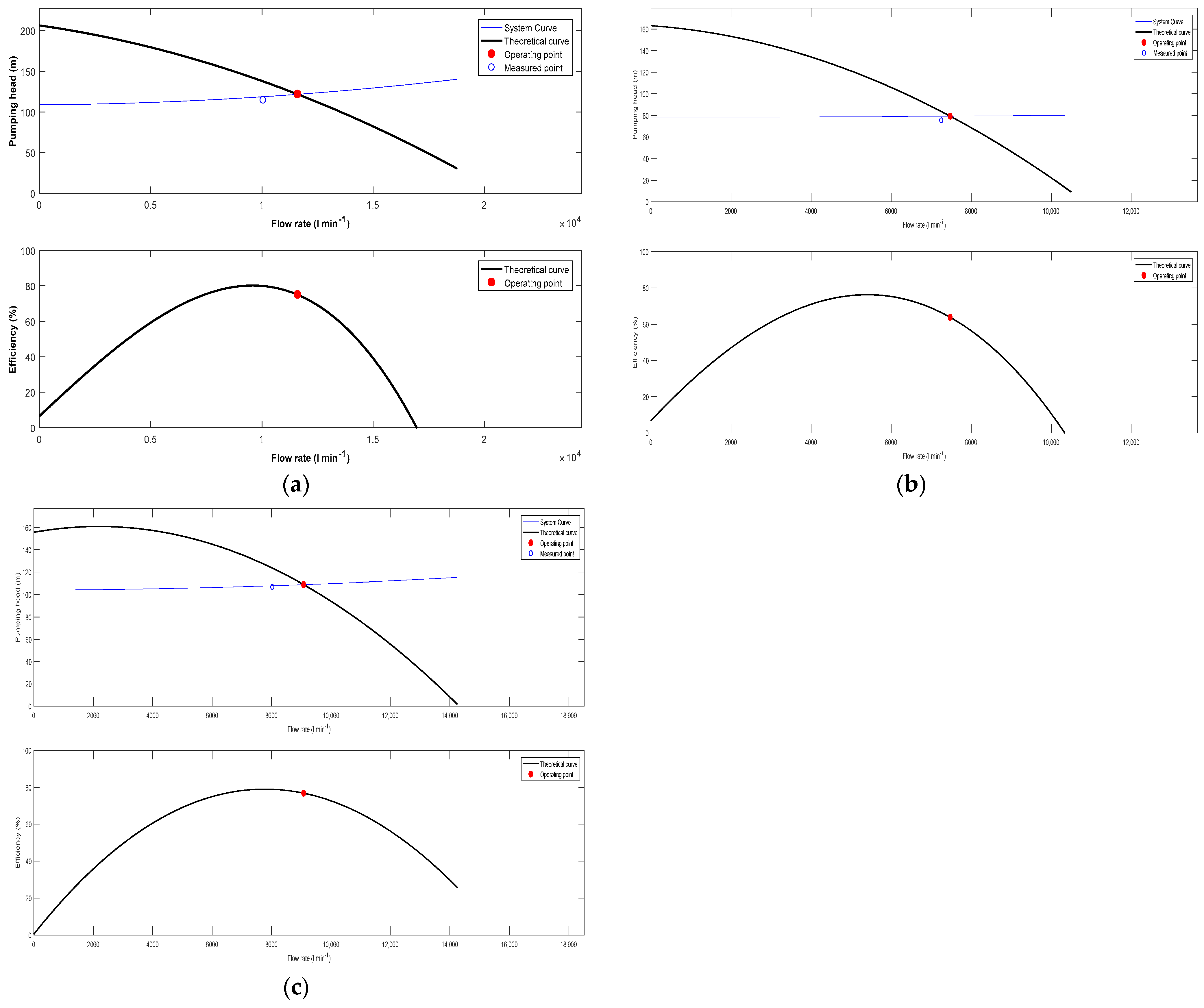
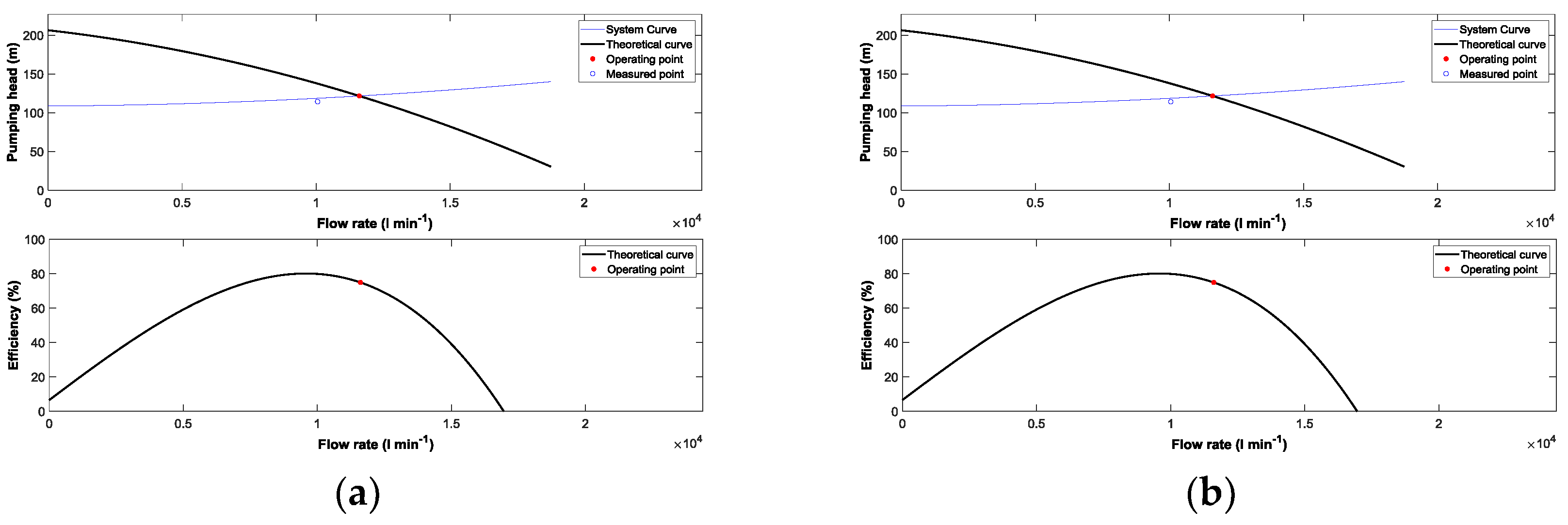
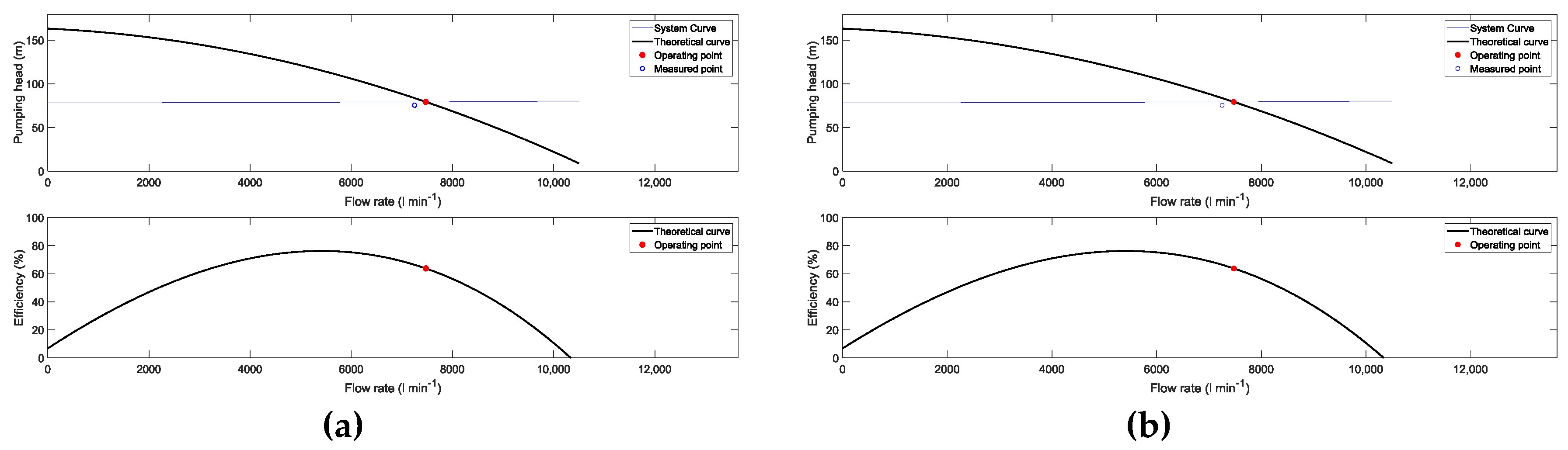
As a first step, the characteristic curves H-Q and efficiency-Q at each one of the analyzed wells are shown in Figure 3. In this case, the theoretical operating point and the measured operating point for the peak period (Case 1) of irrigation season 2007 are shown.
In all the analyzed pumps, the tendency was similar, and it can be highlighted that the operating point did not match with the best efficiency point. It is located instead in a region where the pump efficiency was decreasing. This finding was common in the analyzed WUAs, where the pumps were selected to work in a region where the operating point was located to the right of the maximum efficiency, and the pumps were installed in a way that it was expected to operate in normal conditions. This is related to the fact that the use of underground water resources can increase the water depth level, thereby increasing the dynamic water table (DWT), and increasing the pumping head can lead to the translation of its operating point to a region of maximum efficiency in the nearby future.
In these figures, the measured operating point was included to obtain similar values to the theoretical operating point. With regard to this, these figures are useful to highlight that all the pumps were properly selected and to obtain acceptable efficiency values, which ranged from 64% to 77% in WUA B and WUA C, respectively.
3.2. Piezometer Analysis
One representative piezometer was selected for each analyzed WUA. Two criteria were considered to select each one. First, a proximity criterion to the analyzed well was applied, and the closest piezometers to the analyzed WUA were selected. The second criterion was focused on the piezometer selection with the most available data from several irrigation seasons. In some of the available piezometers, some data were missing; thus, these piezometers were discarded. Therefore, the piezometers with the most available data were then determined.
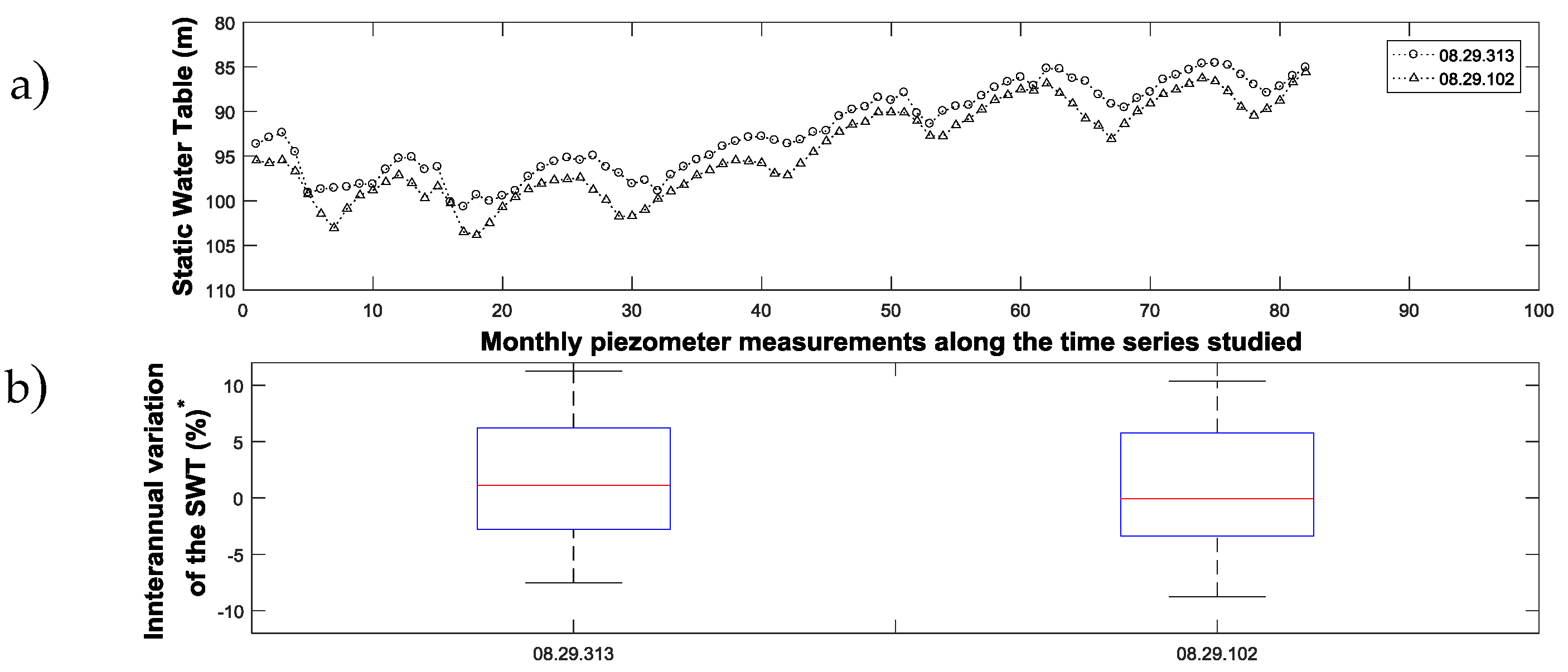
In Figure 4, the evolution of the static water table (SWT) throughout all of the available irrigation seasons is represented at each piezometer, as well as the interannual variation of the SWT with respect to January of 2007. The SWT evolution of the two piezometers (08.29.102 and 08.29.313) of the WUA A is shown in Figure 4a. Both piezometers show a similar tendency, ranging in SWT values from 103 to 85 m. The interannual variation of the SWT values also showed a similar tendency, considering the range of values from 2007 to 2013 (Figure 5b). In this case, piezometers 08.29.313 and 08.29.102 were located at a distance of 9.6 and 12.3 km, respectively. According to the second selection criterion, piezometer 08.29.313 was chosen.
Concerning to WUA B (Figure 5a,b), the SWT evolution remains similar for the three piezometers ranging their SWT values from 62 to 70 m. In this irrigation society, although piezometer 08.29.047 was the closest to the analyzed well, it was located in a region close to a river; thus, the influence of this could affect to the data accuracy. Hence, in this area, piezometer 08.29.051 was selected, which was at a distance of 8.4 km.
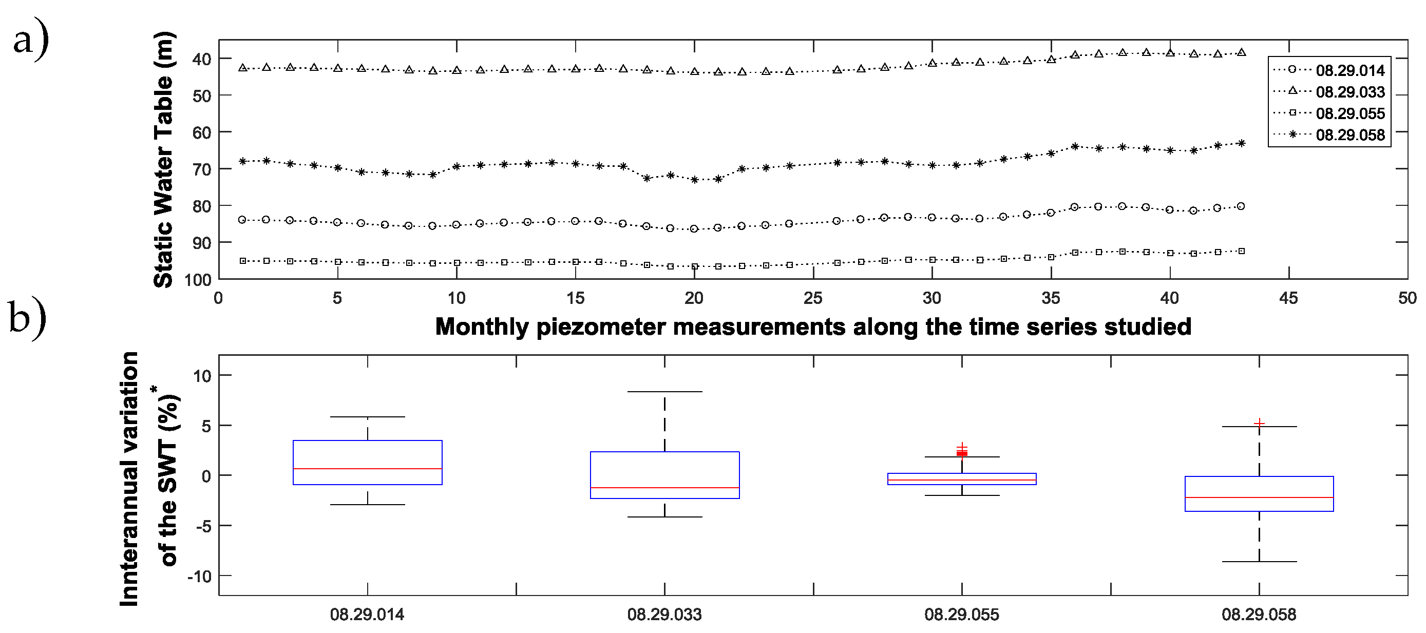
For WUA C, the piezometer 08.29.058 (Figure 6a) had a different tendency in comparison to the other piezometers. In fact, it was too far (25 km) from the analyzed well and was; therefore, discarded. Piezometer 08.29.033 was discarded because it was close to a river. Considering the remaining piezometers with a similar tendency, piezometer 08.29.014 was selected because it is close to the well (distance of 7.5 km) and more information was available for it (Figure 6b).
In Table 4, the DWT for each analyzed case and irrigation season is shown for each of the selected piezometers. In addition, during each irrigation season, the average values of the DWT for each case, along with the coefficient of variation (CV) for each one, is shown. Regarding the CV, it can highlight the low variability of the DWT, considering the selected months for each analyzed case.
For each one of the selected piezometers, the high interannual variation of the DWT can be highlighted. This fact is important because it allows for a wide range of DWT values for each WUA, which is useful for validating the behavior and performance of the developed tool under different dynamic water table levels. Moreover, the selected piezometers show similar tendencies of decreasing the DWT level for the 2011 irrigation season. This fact is explained by the increasing energy tariffs during that period, which resulted in a reduction of the use of groundwater resources in these areas, thereby contributing to the recovery of the aquifers. Hence, several values for the DWT have been used in these WUAs, which are representative of the DWT levels in the Castilla–La Mancha region.
3.3. Energy Analysis
For each analyzed well of each WUA, the irrigation season with the highest DWT value and the last irrigation season whose DWT values are available were chosen for the energy analysis. The DWT levels in Case 3 for the three WUAs analyzed were very similar. Therefore, only Case 1 and Case 2 were considered for the energy analysis of the three WUAs studied. Consequently, for each WUA studied, two irrigation seasons and two cases (Case 1 and Case 2) were considered in this analysis. The irrigation seasons with highest DWT values and the last irrigation season with available data for WUA A, B, and C were 2008, 2007, and 2007; and 2015, 2015, and 2013, respectively.
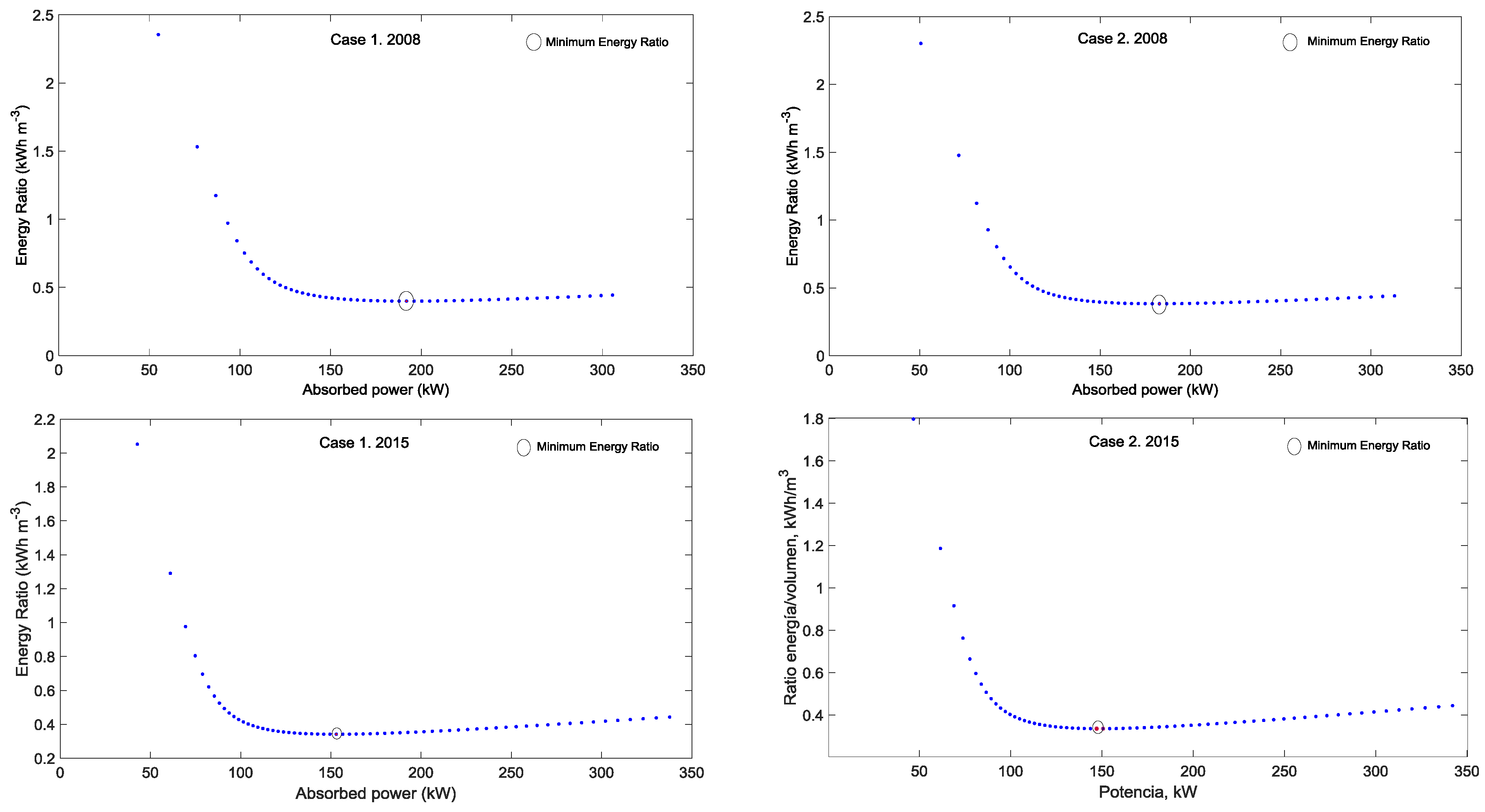
Figure 7, Figure 8, Figure 9, Figure 10, Figure 11, Figure 12, Figure 13, Figure 14 and Figure 15 show the energy analysis results for each WUA, each irrigation season and each studied case. In WUA A (Figure 7), the operating point that minimizes the energy ratio (ER) is shown for Case 1 and Case 2, for irrigation seasons 2008 and 2015. Both irrigation seasons were proposed because of the high difference between the DWT levels among them in each case (Table 4). The minimum ER values reached a value close to 0.399 (Case 1) and 0.373 kWh m−3 (Case 2), which represented variable speed ratios (α) of 0.90 and 0.86, respectively. With regard to the 2015 irrigation season, the minimum ER ranged from 0.342 and 0.336 kWh m−3 for Case 1 and Case 2, respectively, which were obtained for α = 0.82 in both of them.
In 2008, when comparing the ER obtained with a fixed speed (at maximum α) and the variable speed pump that minimized the ER, the maximum energy saving obtained ranged from 9.9% (Case 1) to 13.1% (Case 2). Regarding the 2015 irrigation season, additional differences can be highlighted, with energy savings close to 22.8% (Case 1) and 24.4% (Case 2). In 2008, the difference between the efficiency at α = 1 and α that minimizes the ER was not too high and was more important for the 2015 irrigation season. These differences can be explained when the pump efficiency at each variable speed ratio is represented (Figure 9), where the maximum pump efficiency could not be reached at a fixed speed. This finding is related to the fact that when the pump is working at a fixed speed, the operating point is located to the right of the maximum efficiency, as can be shown in Figure 9 for Case 2. Therefore, when the pump works at a variable speed, the operating point moves to the left, thus increasing the pump efficiency when a variable speed drive is used.
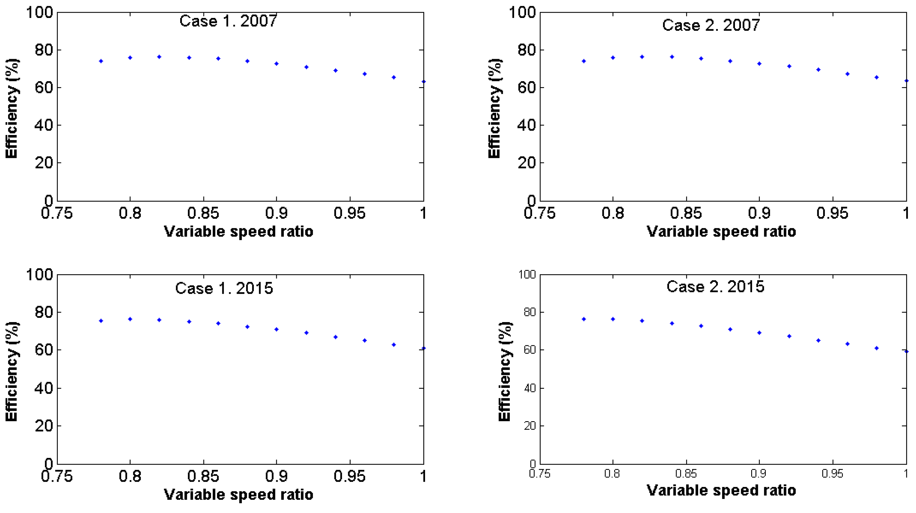
About WUA B, the results for the 2007 and 2015 irrigation seasons are shown. In 2007, no great differences between the ER at fixed speeds and α are shown for Case 1 and Case 2 (Figure 10), which is related to the fact that the DWT level was very similar during the 2007 irrigation season in both of cases. The minimum energy consumed was obtained when a variable speed of 0.82 was used, obtaining energy savings approximately 17.7% and 17.2% in Case 1 and Case 2, respectively, with respect to α = 1. According to this, the minimum ER reached values close to 0.278 and 0.280 kWh m−3 for Case 1 and Case 2, respectively. In both cases, the α value that minimizes ER was close to 0.82. In 2015, the minimum ER was reached for α of 0.80 (Case 1) and 0.78 (Case 2), with ER values of 0.266 (Case 1) and 0.257 kWh m−3 (Case 2), respectively, obtaining energy savings between 20.7% and 23.0%, respectively. In both cases and irrigation seasons, the difference between the pump efficiency at maximum α and the pump efficiency for α that minimizes the ER was high (Figure 11), which is explained for WUA A, because when the pump was working at a fixed speed, the operating points for Case 1 and Case 2 were located to the right of the efficiency curve (Figure 12).
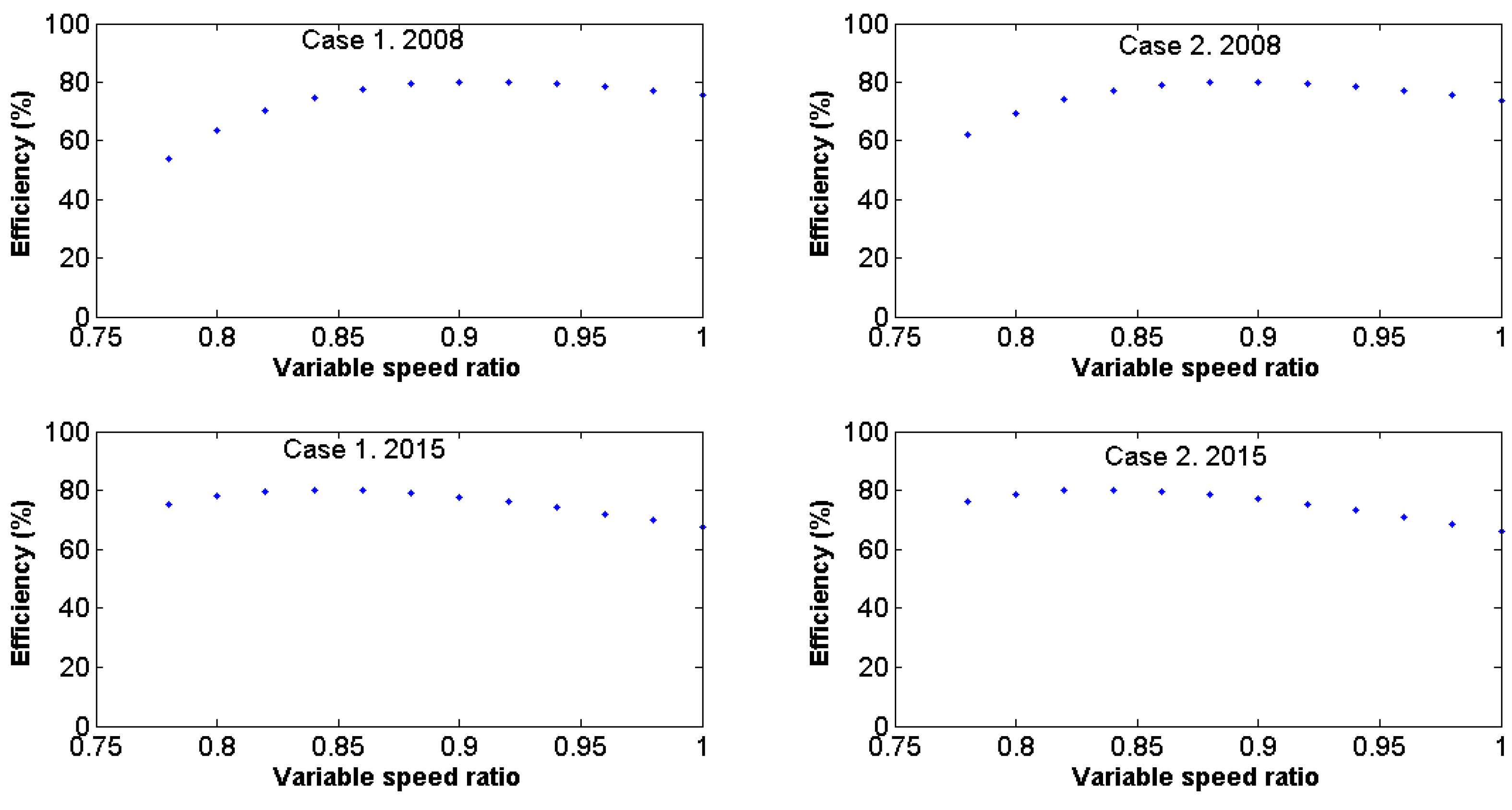
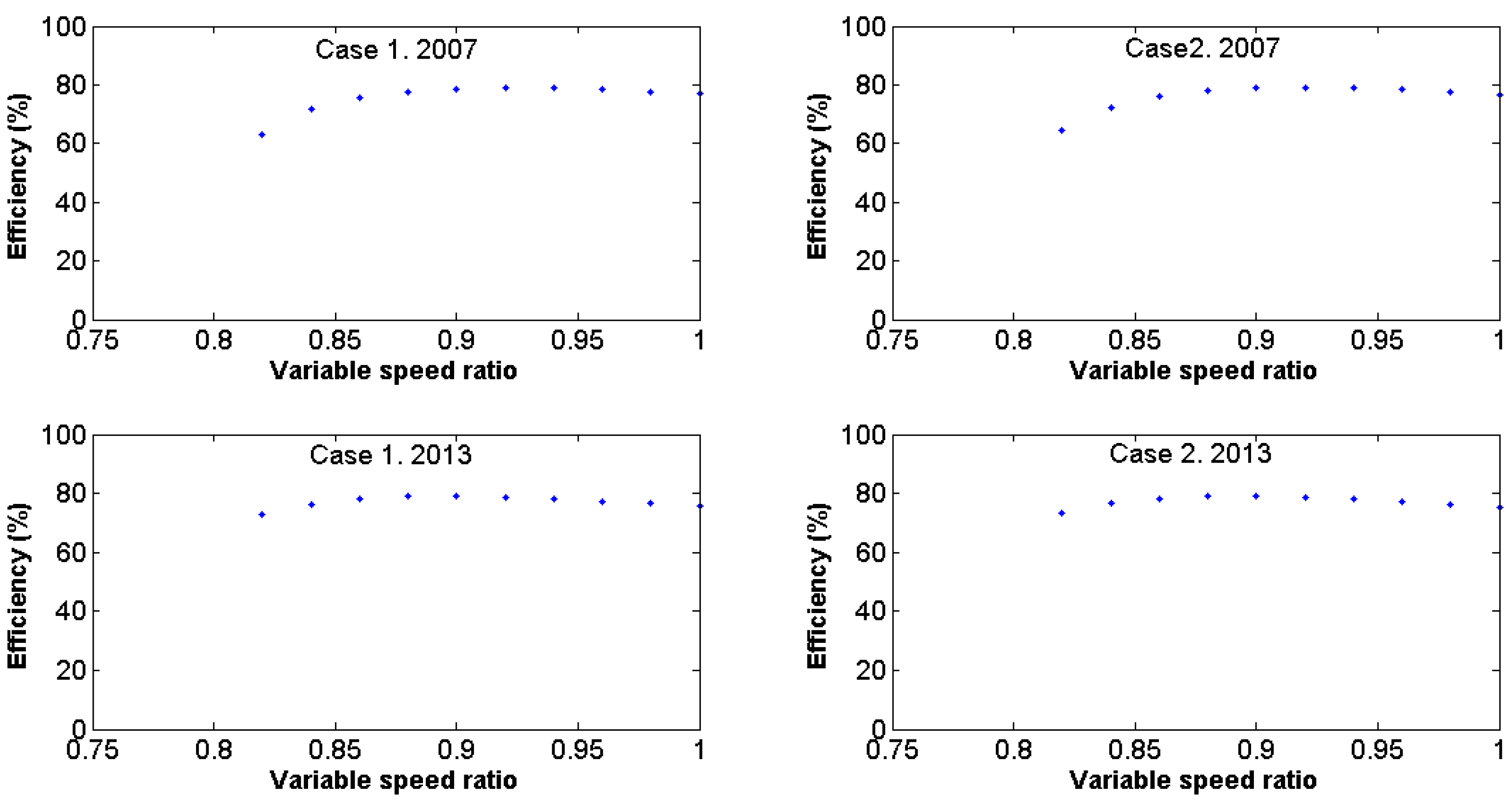
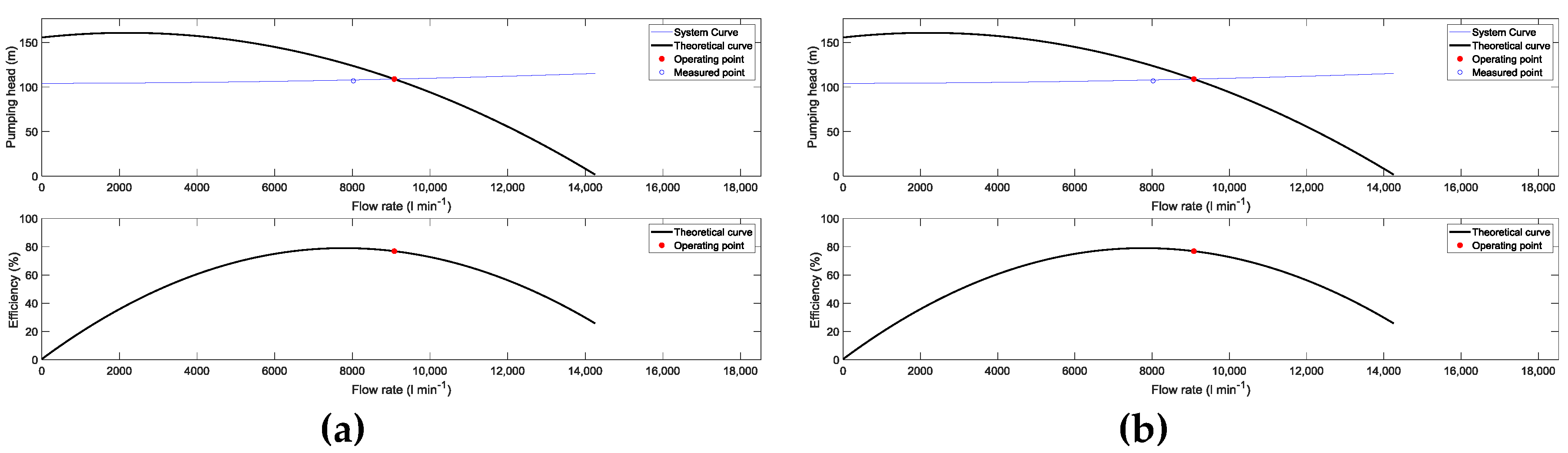
For WUA C, the tendency was very similar to the previously analyzed WUA. In 2007, the variable speed that minimizes the energy consumed per unit of water supplied was 0.9, for Case 1 and Case 2 (Figure 13), and the energy savings obtained ranged from 4.4% and 4.6%, respectively. In 2015, the energy savings slightly increased, ranging from 6.7% (Case 1) to 6.9% (Case 2), and were obtained when comparing the fixed speed with α of 0.88, which minimizes the ER. In both irrigation seasons and analyzed cases, the pump efficiency reached the highest values at a speed ratio of 0.9 (Figure 14), which contributes the energy savings obtained when using a variable speed. The operating point in Case 2 for both irrigation seasons (Figure 15) was to the right of the maximum efficiency, which was similar to that of WUAs A and B.
3.4. Economic Analysis
The economic analysis module assesses the profitability of installing a frequency speed drive vs. the option of a fixed speed. Thus, the speed variable drive investment was evaluated for each study case, irrigation season, and WUA. Table 5 shows a summary of the energy consumed by the fixed speed pump and the variable speed pump, its energy savings, and the absorbed power of the variable speed drive, which determines its investment costs according to equation 5 and the unit energy cost according to the study region. The energy savings obtained by the energetic module of the DSSW tool considering the use of variable speed pumps ranged from 9.9% to 24.4% for WUA A, from 17.2% to 23.0% for WUA B, and from 4.4% to 6.9% for WUA C. The energetic module of the DSSW tool also computes the absorbed power by each speed variable drive. Thus, the absorbed power and the investment cost of the variable speed drive according to equation 5 for WUA A were 371 kW and 23,510 €, respectively. Similarly, the absorbed power of the variable speed drive for WUA B and WUA C were 198 and 251 kW, respectively. The investment cost was 14,344 € for WUA B and 17482 € in the case of WUA C.
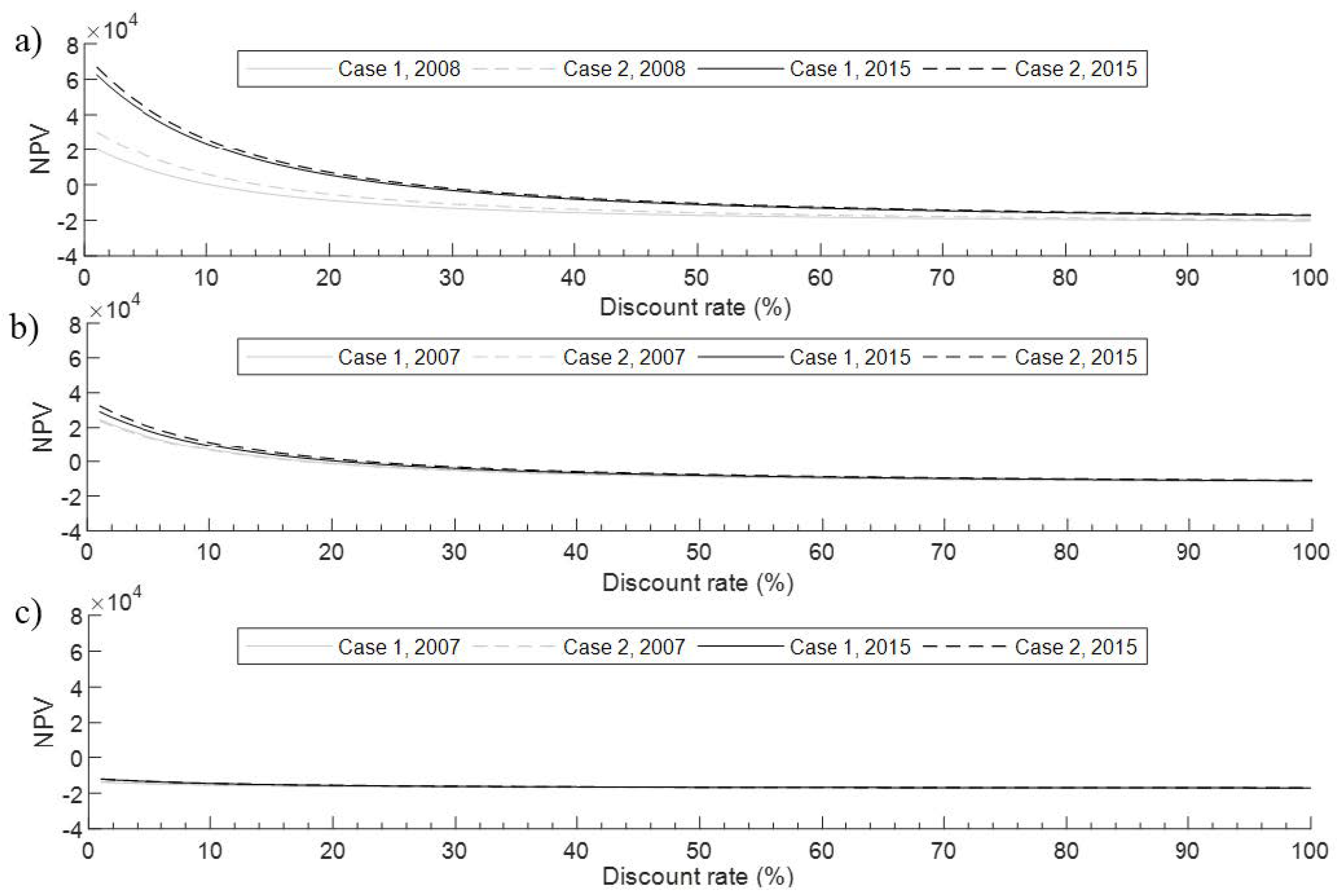
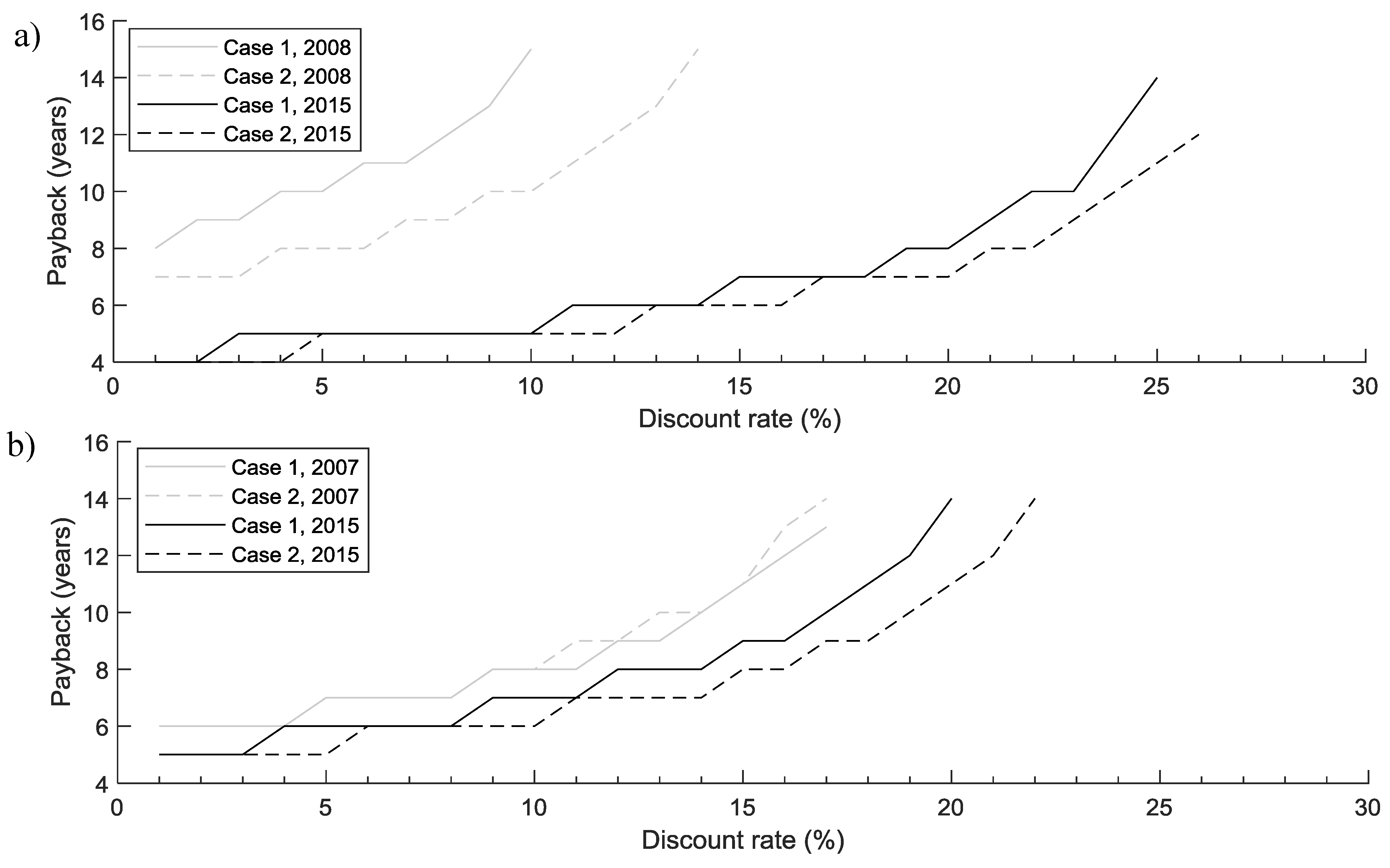
Based on the data shown in Table 5, the economic module of the DSSW tool computes the net present value, NPV (in €), the internal rate of return, IRR, and the payback of each speed variable drive investment. Figure 16 shows the NPV values considering a discount rate which ranged from 1% to 100% (step 1%) for each study case, irrigation season, and WUA A (Figure 16a), WUA B (Figure 16b), and WUA C (Figure 16c). Concerning WUA A, the IRR values were 10% (Case 1) and 14% (Case 2) in 2008 and 26% (Case 1) and 27% (Case 2) in 2015. IRR is the discount rate that makes the NPV of all cash flows equal to zero. Furthermore, an NPV value equal to or higher than zero determines the profitability of potential investments. Consequently, higher NPV values with higher profitability is an investment, and a higher IRR value is the safer investment. The current discount rate is approximately 4.5%, which is far under the IRR value obtained for WUA A. Thus, the investment of the variable speed drive in the WUA A is very cost-effective and safely obtains NPV values for the current discount rate of 10,285, 18,218, 43,188, and 46,617 € for the two case studies and the two irrigation seasons analyzed, respectively, for the 15-year lifespan. The payback periods for the current discount rate were 10, 8, 5, and 4.5 years (Figure 17a).
Regarding the WUA B, in 2007, the IRR values were 18% for Case 1 and Case 2, whereas in 2015, they were 21% (Case 1) and 22% (Case 2). Consequently, although the percentages of energy savings between WUA A and WUA B were similar, the investment safety in WUA B was higher than that of WUA A, and the payback was lower (Figure 17b). These results are because the absorbed power by the variable speed drive in WUA B was much lower than that of WUA A, so the investment cost of the variable speed drive was also lower. Therefore, the NPV values for a discount rate of 4.5% were 15,861, 15,291, 19,376, and 21,988 € for the two case studies and the two irrigation seasons analyzed, respectively, for the 15-year lifespan. Because of the lower energy savings and the lower water volume applied in WUA B, the profitability was smaller. The payback periods for the current discount rate in WUA B were 6.5, 6.5, 6, and 5 years, respectively (Figure 17b).
However, because of the high absorbed power and the high cost of the variable speed drive in WUA C, and the low energy savings and the small amount of water applied, the NPV was negative for any discount rate considered (Figure 16c). Consequently, under the conditions of WUA C, the variable speed drive was unprofitable for the two case studies and the two irrigation seasons analyzed, respectively, for the 15-year lifespan.
4. Conclusions
A decision support system tool for water abstraction from aquifers for irrigation, the DSSW tool, was developed. The proposed tool can be useful for managers of irrigable areas once the crop distribution is known. The proposed methodology can be useful for reducing energy consumption during the water abstraction process from an aquifer to a reservoir in existing wells by installing a frequency speed drive. This tool might be combined with other tools focused on a centralized management, such as Irrigation Advisory Services, where managers can determine the optimum amount of water applied depending on the crop production costs and gross margin. It should be combined with tools that take into account the crop water demands and which give information about the influence of the water applied on crop yields. In this regard, according to the irrigation strategy followed at each area, and the total volume water supplied by wells, managers can decide whether a variable speed drive is or is not profitable.
In the three analyzed cases, energy savings, in comparison with the fixed speed, ranged from 4.4% and 24.4%, using a variable speed ratio of 0.9 and 0.82. The energy savings when using a variable speed frequency increased when the dynamic water table level was lower, and average energy savings close to 23%, 22%, and 6.8% were obtained for irrigation societies A, B, and C, respectively.
An economic analysis module was also developed in the DSSW tool. This module determines the economic profitability of the variable speed drive investment. The results show that the investment cost of the variable speed drive in most irrigation societies studied was very profitable, with a payback that ranged from 4.5 to 10 years. However, irrigation societies with very low energy savings and a high investment cost of the variable speed drive were linked to a low amount of applied water volume, and the investment was unprofitable. This decision support system tool has the potential to be useful for facilitating the transference of this methodology to engineers and managers of irrigable areas.
Author Contributions
Conceptualization, M.A.M. and J.I.C.; methodology, A.I. and R.G.P.; software, J.I.C.; validation, A.I., J.I.C. and R.G.P.; formal analysis, J.I.C., R.G.P., A.I. and, M.A.M.; investigation, J.I.C., R.G.P., A.I. and, M.A.M.; resources, J.I.C. and M.A.M.; data curation, J.I.C. and A.I.; writing—original draft preparation, J.I.C., R.G.P., A.I. and, M.A.M.; writing—review and editing, J.I.C. and R.G.P.; visualization, J.I.C., A.I. and R.G.P.; supervision, M.A.M.; project administration, M.A.M.; funding acquisition, M.A.M.
Funding
We would like to acknowledge the Spanish Ministry of Education and Science (MEC) for funding the AGL2007-66716-C03-03 project and the Consejería de Educación y Ciencia de Castilla-La Mancha for funding the project PCI08-0117. The authors wish also to express their gratitude to the Regional Agency of Energy in Castilla-La Mancha (AGECAM) for funding the project “Auditorías energéticas en Castilla-La Mancha”, contributing funding and support that made the development of this study possible.
Conflicts of Interest
The authors declare no conflict of interest.
References
- Carrión, F.; Sanchez-Vizcaino, J.; Corcoles, J.I.; Tarjuelo, J.M.; Moreno, M.A. Optimization of groundwater abstraction system and distribution pipe in pressurized irrigation systems for minimum cost. Irrig. Sci. 2016, 34, 145–159. [Google Scholar] [CrossRef]
- Moreno, M.A.; Córcoles, J.I.; Moraleda, D.A.; Martinez, A.; Tarjuelo, J.M. Optimization of underground water pumping. J. Irrig. Drain. Eng. 2010, 136, 414–420. [Google Scholar] [CrossRef]
- Khadra, R.; Moreno, M.A.; Awada, H.; Lamaddalena, N. Energy and Hydraulic Performance-Based Management of Large-Scale Pressurized Irrigation Systems. Water Resour. Manag. 2016, 30, 3493–3506. [Google Scholar] [CrossRef]
- Lima, F.A.; Martínez-Romero, A.; Tarjuelo, J.M.; Córcoles, J.I. Model for management of an on-demand irrigation network based on irrigation scheduling of crops to minimize energy use Part I): model Development. Agric. Water Manag. 2018, 210, 49–58. [Google Scholar] [CrossRef]
- Córcoles, J.I.; de Juan, J.A.; Ortega, J.F.; Tarjuelo, J.M.; Moreno, M.A. Management evaluation of Water Users Associations using benchmarking techniques. Agric. Water Manag. 2010, 98, 1–11. [Google Scholar] [CrossRef]
- Córcoles, J.I.; De Juan, J.A.; Ortega, J.F.; Tarjuelo, J.M.; Moreno, M.A. Evaluation of Irrigation Systems by Using Benchmarking Techniques. J. Irrig. Drain. Eng. 2012, 138, 225–234. [Google Scholar] [CrossRef]
- Rodríguez Díaz, J.A.; López Luque, R.; Carrillo Cobo, M.T.; Montesinos, P.; Camacho Poyato, E. Exploring energy saving scenarios for on-demand pressurised irrigation networks. Biosyst. Eng. 2009, 104, 552–561. [Google Scholar] [CrossRef]
- Carrillo Cobo, M.T.; Rodríguez Díaz, J.A.; Montesinos, P.; López Luque, R.; Camacho Poyato, E. Low energy consumption seasonal calendar for sectoring operation in pressurized irrigation networks. Irrig. Sci. 2011, 29, 157–169. [Google Scholar] [CrossRef]
- Fernández García, I.; Moreno, M.A.; Rodríguez Díaz, J.A. Optimum pumping station management for irrigation networks sectoring: Case of Bembezar MI (Spain). Agric. Water Manag. 2014, 144, 150–158. [Google Scholar] [CrossRef]
- González Perea, R.; Camacho Poyato, E.; Montesinos, P.; Rodríguez Díaz, J.A. Critical points: Interactions between on-farm irrigation systems and water distribution network. Irrig. Sci. 2014, 32, 255–265. [Google Scholar] [CrossRef]
- Rodríguez Díaz, J.A.; Montesinos, P.; Camacho Poyato, E. Detecting Critical Points in On-Demand Irrigation Pressurized Networks—A New Methodology. Water Resour. Manag. 2012, 26, 1693–1713. [Google Scholar] [CrossRef]
- Jiménez-Bello, M.A.; Martínez-Alzamora, F.; Castel, J.R.; Intrigliolo, D. Validation of a methodology for grouping intakes of pressurized irrigation networks into sectors to minimize energy consumption. Agric. Water Manag. 2011, 102, 46–53. [Google Scholar] [CrossRef] [Green Version]
- Córcoles, J.I.; Tarjuelo, J.M.; Moreno, M.A. Methodology to improve pumping station management of on-demand irrigation networks. Biosyst. Eng. 2016, 144, 94–104. [Google Scholar] [CrossRef]
- Moreno, M.A.; Ortega, J.F.; Córcoles, J.I.; Martínez, A.; Tarjuelo, J.M. Energy analysis of irrigation delivery systems: Monitoring and evaluation of proposed measures for improving energy efficiency. Irrig. Sci. 2010, 28, 445–460. [Google Scholar] [CrossRef]
- Helweg, O.J. DETERMINING OPTIMAL WELL DISCHARGE. ASCE J Irrig Drain Div 1975, 101, 201–208. [Google Scholar]
- Scalmanini, J.C.; Scott, V.H.; Helweg, O.J. Energy and efficiency in wells and pumps. Proc. 12th Bienn. Conf. Gr. Water, Sacramento, Calif. Calif. Water Resour. Cent. Rep. 1979, 45, 1–210. [Google Scholar]
- Helweg, O.J.; VonHofe, F.; Quek, P.T. Improving well hydraulics. In Proceedings of the Irrigation Drainage Special Conference, Honolulu, HI, USA, 22–24 July 1991. [Google Scholar]
- Helweg, O.J.; Jacob, K.P. Selecting the optimum discharge rate for a water well. Hydraul. Eng. 1991, 117, 934–939. [Google Scholar] [CrossRef]
- Moreno, M.A.; Medina, D.; Ortega, J.F.; Tarjuelo, J.M. Optimal design of center pivot systems with water supplied from wells. Agric. Water Manag. 2012, 107, 112–121. [Google Scholar] [CrossRef]
- Domínguez, A.; Martínez, R.S.; Juan, J.A.; Martínez-Romero, A. Simulation of maize crop behaviour under deficit irrigation using MOPECO model in a semi-arid environment. Agric. Water Manag. 2012, 107, 42–53. [Google Scholar] [CrossRef]
- Lamaddalena, N.; Sagardoy, J.A. Performance analysis of on-demand pressurized irrigation systems; FAO: Rome, Italy, 2000; Volume 132. [Google Scholar] [CrossRef]
- Calejo, M.J.; Lamaddalena, N.; Teixeira, J.L.; Pereira, L.S. Performance analysis of pressurized irrigation systems operating on-demand using flow-driven simulation models. Agric. Water Manag. 2008, 95, 154–162. [Google Scholar] [CrossRef]
Figure 1.
Infrastructure of the analyzed system.

Figure 2.
Location of the piezometers and analyses at Irrigation Society A (a), B (b), and C (c).

Figure 3.
Characteristic curves H-Q, efficiency-Q, and operating point for Case 1 in WUA A (a), B (b), and C (c).
Figure 3.
Characteristic curves H-Q, efficiency-Q, and operating point for Case 1 in WUA A (a), B (b), and C (c).

Figure 4.
Static water table (a) and monthly interannual variation (b) for each piezometer in WUA A.
Figure 4.
Static water table (a) and monthly interannual variation (b) for each piezometer in WUA A.

* Interannual variation of the SWT1 with respect to January of 2007. 1Static Water Table
Figure 5.
Static water table (a) and monthly interannual variation (b) for each piezometer in WUA B.
Figure 5.
Static water table (a) and monthly interannual variation (b) for each piezometer in WUA B.

* Interannual variation of the SWT with respect to January of 2007
Figure 6.
Static water table (a) and monthly interannual variation (b) for each piezometer in WUA C.
Figure 6.
Static water table (a) and monthly interannual variation (b) for each piezometer in WUA C.

* Interannual variation of the SWT with respect to January of 2007
Figure 7.
Energy ratio (kWh m−3) at each variable speed ratio (α) in WUA A.

Figure 8.
Pump efficiency (%) depending on the variable speed ratio in WUA A.

Figure 9.
Operating point at fixed speed in WUA A for Case 2 in 2008 (a) and 2015 (b) irrigation seasons.
Figure 9.
Operating point at fixed speed in WUA A for Case 2 in 2008 (a) and 2015 (b) irrigation seasons.

Figure 10.
Energy ratio (kWh m−3) at each variable speed ratio (α) in WUA B.

Figure 11.
Pump efficiency (%) depending on the variable speed ratio in WUA B.

Figure 12.
Operating point at fixed speed in WUA B for Case 2 in 2007 (a) and 2015 (b) irrigation seasons.
Figure 12.
Operating point at fixed speed in WUA B for Case 2 in 2007 (a) and 2015 (b) irrigation seasons.

Figure 13.
Energy ratio (kWh m−3) at each variable speed ratio (α) in WUA C.

Figure 14.
Pump efficiency (%) depending on the variable speed ratio in WUA C.

Figure 15.
Operating point at fixed speed in WUA C for Case 2 in 2007 (a) and 2013 (b) irrigation seasons.
Figure 15.
Operating point at fixed speed in WUA C for Case 2 in 2007 (a) and 2013 (b) irrigation seasons.

Figure 16.
Net present value for several discount rates of the speed variable drive investment for WUA A (a), WUA B (b), and WUA C (c).
Figure 16.
Net present value for several discount rates of the speed variable drive investment for WUA A (a), WUA B (b), and WUA C (c).

Figure 17.
Payback period for several discount rates of the speed variable drive investment for WUA A (a) and WUA B (b).
Figure 17.
Payback period for several discount rates of the speed variable drive investment for WUA A (a) and WUA B (b).


Table 1.
Characteristics of the water user associations.
| Irrigation Society | A | B | C |
|---|---|---|---|
| Command area (ha) | 863 | 764 | 267 |
| Wells (number) | 4 | 6 | 1 |
| Storage capacity (m3) | 130,000 | 5 of 5000 1 of 6000 | 20,000 |
| Water distribution network management | Rotational schedule | Rotational schedule | On demand |
| Irrigation system | Sprinkler and drip irrigation | Sprinkler and drip irrigation | Drip irrigation |
Table 2.
General information required by the developed tool.
| Pump Model | WUA* A | WUA B | WUA C |
|---|---|---|---|
| INDAR 423-3 | INDAR BL-345-3 | INDAR BL-385-3 | |
| Reference level of dynamic water table (Zo, mm) | 588.15 | 602.57 | 646.89 |
| Reference level of water discharged (Zf, mm) | 697.00 | 680.10 | 751.03 |
| Pumping pipe diameter (D, mm) | 250 | 315 | 272 |
| Hazen–Williams coefficient (C) at the pumping pipe | 125 | 125 | 125 |
| Pumping pipe length (L, m) | 160 | 100 | 130 |
| Distribution pipe diameter (D, mm) | 588 | 315 | 272 |
| Hazen–Williams coefficient (C) at the distribution pipe | 125 | 125 | 125 |
| Distribution pipe length (L, m) | 2750 | 10 | 50 |
*WUA: Water User Association.
Table 3.
Piezometer information for each irrigated area.
| WUA | Id-Number | Coord X (1) | Coord Y (1) | Data Available (Years) |
|---|---|---|---|---|
| A | 08.29.102 | 585981.8361 | 4304764.2977 | From 2007 to 2013 |
| 08.29.313 | 589075.8342 | 4303205.2979 | ||
| B | 08.29.047 | 600345.1536 | 4334477.9268 | From 2007 to 2013 2015 |
| 08.29.051 | 600729.1332 | 4332226.9447 | ||
| 08.29.060 | 599206.0866 | 4328434.9856 | ||
| C | 08.29.033 | 577548.335 | 4358316.5237 | From 2007 to 2013 |
| 08.29.058 | 556391.9999 | 4344263.9132 | From 2007 to 2013 | |
| 08.29.055 | 573112.1778 | 4347483.7795 | From 2007 to 2011 | |
| 08.29.014 | 577430.1485 | 4346041.8566 | From 2008 to 2013 |
(1) Coordinate system: UTM ETR89.
Table 4.
Average dynamic water table (DWT) and coefficient of variation (CV) for each irrigation season and analyzed case.
Table 4.
Average dynamic water table (DWT) and coefficient of variation (CV) for each irrigation season and analyzed case.
| Piezometer | 2007 | 2008 | 2009 | 2010 | 2011 | 2012 | 2013 | 2015 | ||||||||
|---|---|---|---|---|---|---|---|---|---|---|---|---|---|---|---|---|
| 08.29.313 | DWT (m) | CV (%) | DWT (m) | CV (%) | DWT (m) | CV (%) | DWT (m) | CV (%) | DWT (m) | CV (%) | DWT (m) | CV (%) | DWT (m) | CV (%) | DWT (m) | CV (%) |
| Case 1 | 105.5 | 0.28 | 106.9 | 0.67 | 103.7 | 0.99 | 99.62 | 0.44 | 96.73 | 0.85 | 92.98 | 1.12 | 91.79 | 1.26 | 91.09 | 1.05 |
| Case 2 | 99.70 | 1.20 | 102.5 | 0.76 | 101.7 | 0.26 | 99.80 | 0.54 | 94.43 | 0.50 | 91.75 | 1.28 | 90.68 | 0.50 | 89.44 | 2.64 |
| Case 3 | 105.0 | 0.19 | 106.3 | 0.58 | 104.6 | 0.94 | 98.92 | 0.59 | 95.11 | 0.72 | 95.20 | 0.59 | 93.03 | 1.10 | 92.23 | 0.01 |
| Case 1 | 71.03 | 0.38 | 70.54 | 0.53 | 71.01 | 1.31 | 68.69 | 0.21 | 64.98 | 0.69 | 65.44 | 2.21 | 64.96 | 0.71 | 67.62 | 1.39 |
| Case 2 | 71.52 | 0.57 | 69.80 | 0.13 | 68.78 | 0.34 | 68.70 | 0.71 | 64.42 | 0.72 | 64.05 | 1.05 | 65.56 | 1.18 | 65.00 | 0.23 |
| Case 3 | 71.42 | 0.20 | 71.17 | 0.00 | 71.87 | 0.31 | 68.60 | 0.83 | 66.08 | 0.35 | 68.83 | 0.66 | 66.05 | 0.62 | 69.15 | 0.05 |
| Case 1 | 98.82 | 0.52 | 99.21 | 0.40 | 100.24 | 0.43 | 97.20 | 0.22 | 94.37 | 0.60 | 94.00 | 0.86 | 92.85 | 0.68 | - | - |
| Case 2 | 98.12 | 0.16 | 97.96 | 0.35 | 98.35 | 0.35 | 97.59 | 0.71 | 93.91 | 0.53 | 92.24 | 0.23 | 92.35 | 0.37 | - | - |
| Case 3 | 98.63 | 0.34 | 99.09 | 0.48 | 99.56 | 0.53 | 95.83 | 0.80 | 93.69 | 0.71 | 94.07 | 0.79 | 92.29 | 0.90 | - | - |
Table 5.
Energy consumption of fixed speed pump, variable speed pump, energy saving, absorbed power by the variable speed drive, and investment cost of the variable speed drive.
Table 5.
Energy consumption of fixed speed pump, variable speed pump, energy saving, absorbed power by the variable speed drive, and investment cost of the variable speed drive.
| WUA | Cases | Energy Consumption (kWh m−3) 1 | Energy Consumption (kWh m−3) 2 | Energy Saving (%) | Absorbed Power by the Variable Speed Drive (kW) | Investment Cost of the Variable Speed Drive (€) |
|---|---|---|---|---|---|---|
| A | Case 1, 2008 | 0.439 | 0.399 | 9.92 | 371 | 23,510 |
| Case 2, 2008 | 0.422 | 0.373 | 13.10 | 371 | 23,510 | |
| Case 1, 2015 | 0.420 | 0.342 | 22.84 | 371 | 23,510 | |
| Case 2, 2015 | 0.418 | 0.336 | 24.44 | 371 | 23,510 | |
| B | Case 1, 2007 | 0.327 | 0.278 | 17.7 | 198 | 14,344 |
| Case 2, 2007 | 0.328 | 0.280 | 17.24 | 198 | 14,344 | |
| Case 1, 2015 | 0.321 | 0.266 | 20.65 | 198 | 14,344 | |
| Case 2, 2015 | 0.316 | 0.257 | 23.03 | 198 | 14,344 | |
| C | Case 1, 2007 | 0.387 | 0.371 | 4.35 | 251 | 17,482 |
| Case 2, 2007 | 0.385 | 0.368 | 4.64 | 251 | 17,482 | |
| Case 1, 2015 | 0.372 | 0.349 | 6.70 | 251 | 17,482 | |
| Case 2, 2015 | 0.372 | 0.348 | 6.90 | 251 | 17,482 |
1 Energy consumption of fixed speed pump. 2 Energy consumption of variable speed pump.
© 2019 by the authors. Licensee MDPI, Basel, Switzerland. This article is an open access article distributed under the terms and conditions of the Creative Commons Attribution (CC BY) license (http://creativecommons.org/licenses/by/4.0/).
Share and Cite
MDPI and ACS Style
Córcoles, J.I.; Gonzalez Perea, R.; Izquiel, A.; Moreno, M.Á. Decision Support System Tool to Reduce the Energy Consumption of Water Abstraction from Aquifers for Irrigation. Water 2019, 11, 323. https://doi.org/10.3390/w11020323
AMA Style
Córcoles JI, Gonzalez Perea R, Izquiel A, Moreno MÁ. Decision Support System Tool to Reduce the Energy Consumption of Water Abstraction from Aquifers for Irrigation. Water. 2019; 11(2):323. https://doi.org/10.3390/w11020323
Chicago/Turabian StyleCórcoles, Juan Ignacio, Rafael Gonzalez Perea, Argenis Izquiel, and Miguel Ángel Moreno. 2019. "Decision Support System Tool to Reduce the Energy Consumption of Water Abstraction from Aquifers for Irrigation" Water 11, no. 2: 323. https://doi.org/10.3390/w11020323
Note that from the first issue of 2016, this journal uses article numbers instead of page numbers. See further details here.