Deciphering Interannual Temperature Variations in Springs of the Campania Region (Italy)


1
Department of Environmental, Biological and Pharmaceutical Sciences and Technologies, University of Campania “Luigi Vanvitelli”, Via Vivaldi 43, 81100 Caserta, Italy
2
Department of Materials, Environmental Sciences and Urban Planning, Polytechnic University of Marche, Via Brecce Bianche 12, 60131 Ancona, Italy
*
Author to whom correspondence should be addressed.
Water 2019, 11(2), 288; https://doi.org/10.3390/w11020288
Submission received: 24 December 2018
/
Revised: 31 January 2019
/
Accepted: 3 February 2019
/
Published: 7 February 2019
(This article belongs to the Special Issue Insights on the Water–Energy–Food Nexus)
Abstract
:While the effects of climate change on the thermal regimes of surface waters have already been assessed by many studies, there is still a lack of knowledge on the effects on groundwater temperature and on the effects on spring water quality. The online available dataset of the Campania Environmental Agency (ARPAC) was analysed via spatial, temporal and statistical analyses to assess the impact of climate variability on 118 springs, monitored over the period from 2002 to 2017. The meteorological dataset was used to compute average annual precipitation and atmospheric temperatures. Spring water temperatures, electrical conductivity, pH, chloride and fluoride were selected to determine if climate variations had a significant impact on spring water quality. This study shows that the Campania region has experienced an increase of spring water temperatures of approximately 2.0 °C during the monitored period. This is well-linked with the increase of atmospheric minimum temperatures, but not with average and maximum atmospheric temperatures. The spring water temperature increases were not reflected by a concomitant change of the analysed water quality parameters. The latter were linked to the precipitation trend and other local factors, like spring altitude and the presence of geothermal heat fluxes.
1. Introduction
The climate on Earth has been continuously changing for billions of years, and will continue to change in the future. The Mediterranean Region has already been impacted by recent climate change, with forecasted temperature increases [1], specifically in the summer seasons [2,3,4], decreasing yearly precipitation, and increasing extreme events [4,5,6]. The main concern raised by climate change is that it will modify the global hydrological cycle (GHC), even if mitigation scenarios are applied [7,8,9]. To date, most research has been done on the atmospheric components of the GHC, both on historical and projected changes [10,11]. Conversely, for the sub-surface components of the GHC (e.g., recharge, groundwater levels, aquifer fluxes and groundwater quality), the conceptual model is still fragmentary, and some of these components have not yet been taken into consideration [12,13].
It is certain that climate change and land use changes will have a manifold effect on groundwater resources, both from a quantitative and qualitative perspective. While research on groundwater availability in view of climate change has gained increasing attention in the last years, studies on future groundwater quality are hard to find in the literature [14]. One of the main drivers affecting groundwater quality evolution with climate change and land use change is temperature. For this reason, new studies dealing with surface water and groundwater temperature change are needed, to properly distinguish between climate and land use change effects on groundwater systems. Once again, the scientific literature on surface historical and forecasted trends is larger than the one for sub-surface trends. Studies of historical changes in river water temperature generally report increases [15]. A recent modelling study on Wisconsin streams suggests that annual average stream temperature will increase 1.1 to 3.2 °C by 2100 [16]. In some cases, changes to the thermal regime can be locally attributed to anthropogenic drivers, but the changes that are pervasive in the river network, are more likely due to climate change [17]. A study from Houben et al. [18] in Germany demonstrated that groundwater temperature data follow air temperature trends remarkably well. This holds true especially for the last 50 years, where both air and groundwater recharge temperatures have shown an increase of 1.5 °C. Menberg et al. [19] demonstrated the direct influence of atmospheric temperature on shallow groundwater temperature at two sites in Germany.
The rise of groundwater temperature by several degrees and the widening of seasonal thermal variations [20] in response to atmospheric temperature changes is widely accepted in the scientific community, but, despite this, the implications of these variations on groundwater chemistry have still not been investigated in detail. The thermal response of groundwater to climate change and land use, as well as the concurrent shift of biogeochemical reactions occurring within the aquifers are relevant not only for groundwater quality but also for surface water, since baseflow-dominated systems and aquifers are inextricably linked [13]. Recently, it has been highlighted that the increase of groundwater temperature in an unconfined aquifer in the Campania region over the last 15 years could be due to the concomitant increase of minimum annual air temperature [21]. Thus, more studies are necessary in this region, as well in other regions, to find clear links between atmospheric temperatures and groundwater regimes. In this paper, a 16 years dataset on air and spring water temperatures and water quality parameters is analysed to unravel if the increase of atmospheric temperatures has induced changes in spring water temperature and quality in the Campania region.
2. Materials and Methods
2.1. Study Area
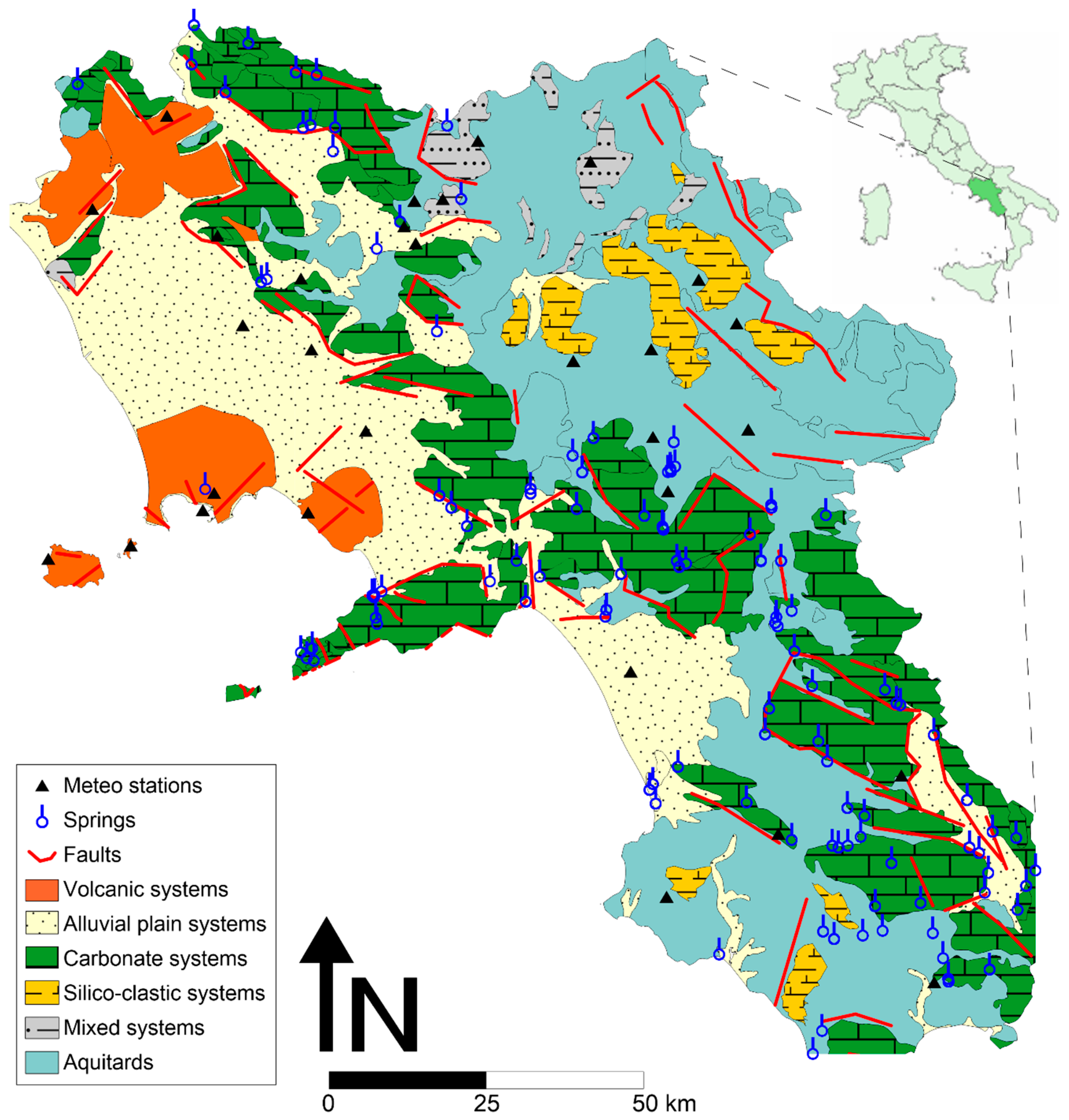
The Campania region is located in the southern Italian Peninsula with a total area of 13.595 km2, surrounded by the Apennine to the west, which occupies a big portion of the territory, and the Tyrrhenian Sea to the east (Figure 1). Morphologically, the Campania region is dominated by the Apennine Mountains and by two large coastal plains: Campana and Sele plains. These two alluvial plains are the result of river activity, and were formed in the place where carbonate units were depressed by tectonic extensive movements [22]. Campania and Sele plains are occupied, respectively, by the two main rivers of the region, the Volturno and the Sele, and are characterized by large land reclamation works. The region has a Mediterranean climate with a cold winter and dry summer, with wetter summers near the coastline and more severe winters in the mountains. There are large differences between mountain and coastal zones, in fact, maximum and minimum temperatures can vary of 6–8 °C between the mountain peaks and the coastal plains [23]. The mean annual rainfalls occur mainly in the period between October and May, showing clear differences in terms of elevation and proximity to the sea. The highest precipitation amounts occur in the Apennine chain, with values of 1200–1500 mm/y, up to 2000 mm/y. Lower values are registered in the coastal plains, with values around 800 mm/y [24]. From a geological point of view, the region is mainly made up of sedimentary and volcanic rocks. The Apennine domain is characterized by sedimentary rocks like limestones, dolomites and terrigenous sediments of Mesozoic age. Theses formation are buried under variable thicknesses of Neogene units, mainly made of volcanoclastic materials from the volcanic districts: the Roccamonfina Volcano in the northwest and from the Somma-Vesuvio and Campi Flegrei districts in the central part of the Campania coast. The plains are characterized by quaternary sediments from fluvial deposition (alluvial and lacustrine deposits).
The Tyrrhenian Sea is the outlet of the watershed, and is the western boundary of the study area. The Campania region comprises many hydrogeological systems: quaternary alluvial deposits, pyroclastic deposits, carbonate karstified systems and silico-clastic systems [25]. High values of hydraulic conductivity characterize the karst aquifers. However, clay formations and marls also occur, especially in the areas located in the central part of the Campania region and near the southern boundary, forming large aquitards (Figure 1). The land use is heterogeneous, with urban areas covering 15% of the area (especially around Naples), while the forested areas cover more than 30% of the territory. The land use is dominated by agricultural fields, covering more than 50% of the territory, with farming activities mainly focused in the coastal plains. The highly populated urban areas are concentrated near the mountain ranges and in the large alluvial plains [26].
2.2. Database Selection
For this study, selected physiochemical properties of water in 118 monitored springs (see Figure 1 for location) from the online available dataset of ARPAC (Agenzia Regionale per la Protezione Ambientale in Campania) [27] were considered. Among the large database available on spring water quality parameters, temperature, electrical conductivity (EC), pH, chloride (Cl−) and fluoride (F−) were selected to determine if the climate variations recorded during the available monitoring period (from 2002 to 2017) had a significant impact on spring water physiochemical parameters (Table 1). EC and pH were selected since they describe the dissolved ions in solution, and they are often influenced by recharge processes, while Cl− and F− were selected since they are non-reactive and reactive environmental tracers, respectively. Each spring was monitored three times for years; some missing period of analysis are probably due to system maintenance or malfunctions. The EC, pH, Cl− and F− observed data from all the available springs were used to generate mean yearly data and to calculate the respective standard deviations. The total number of spring water temperatures, EC, pH, Cl− and F− data analysed were 1354, 1396, 1156, 1528 and 936, respectively. Temperature, EC and pH were measured in situ, while Cl− and F− were collected in HDPE bottles and analysed in a laboratory using standard techniques. There were 32 online available meteorological stations (see Figure 1 for location) with daily precipitations, minimum, maximum and mean air temperatures from 2002 to 2007 [28]. The daily observed data were used to generate mean yearly data on air temperatures and precipitations from 2002 to 2007, while the data from 2008 to 2017 are available online from the Ministry of Agriculture website [29]. The use of an index representative of the annual temperature anomaly is more appropriate for assessing the climate trend at a regional scale, since it minimizes variations due to local factors [30]. Thus, a regional mean annual air temperature index (MATI) and a regional mean annual precipitation index (MAPI) were calculated following the procedure explained in De Vita et al. [30].
2.3. Statistical Analyses
The spring water dataset was initially analysed using both multiple linear regression and Pearson correlation and ANOVA tests via Excel 2016 (Microsoft, Redmond, WA, USA). A multivariate statistical analysis was then performed to identify possible correlations between the spring water parameters. Efficient multivariate statistical tools that have been successfully applied for groundwater [31], surface and springs water [32] are factor analysis (FA) and principal component analysis. For this work, FA was chosen and applied to reduce a large number of variables into fewer numbers of factors, extracting maximum common variance from all variables and putting them into a common score. The relationship of each variable to the underlying factor is expressed by the so-called factor loading, which shows the variance explained by the variable of that particular factor. Level of meaningfulness was done by the Kaiser–Meyer–Olkin (KMO) method, and had to be higher than 0.5 [33]. FA does not replace a univariate approach, which is necessary for explorative analyses of the data, but is useful when simplification, classification, systematization and model building is needed. The spatial analysis of spring parameters was performed using the classed post-map tool of Surfer 16.0 (Golden Software, Golden, CO, USA). Each parameter was subdivided into five equal intervals classes to better visualize spatial variations.
3. Results and Discussion
3.1. Recorded Yearly Temperature and Precipitation Variations
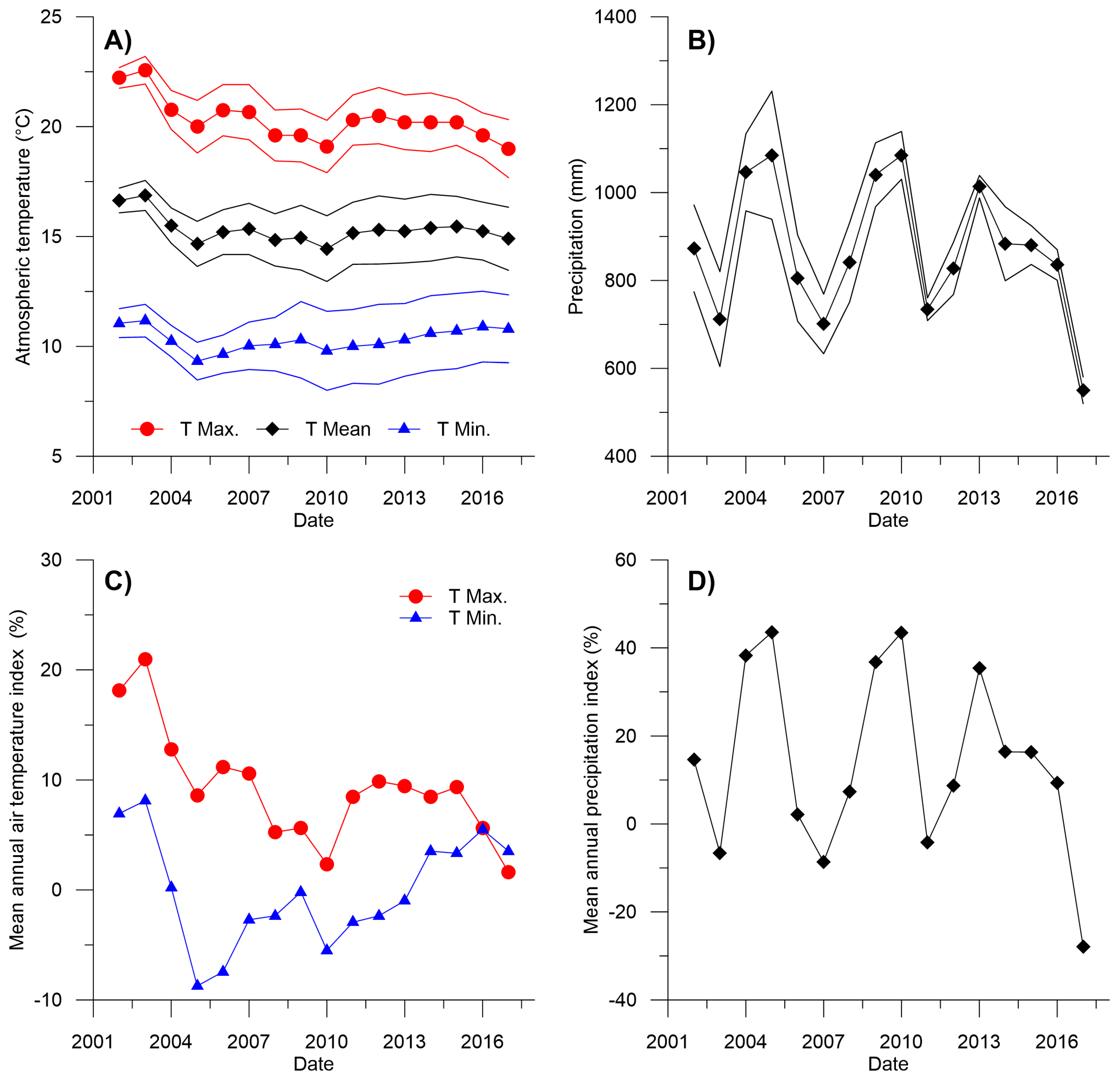
Figure 2 shows the trend of yearly averaged maximum and minimum air temperatures in the Campania region during the period 2002–2017. The maximum air temperatures exhibit a slightly decreasing trend of approximately −0.14 °C/y, although an oscillating trend is recognizable in the series, which decreased the overall fit with linear interpolation to R2 of 0.46.
The minimum air temperatures trend has an even worst R2 of 0.03, when the whole dataset is employed. On the contrary, the minimum air temperatures exhibit a clear increasing trend of +0.11 °C/y, with an R2 of 0.81 using the dataset from 2005 to 2017. Clearly, the mean air temperature trend lies between the maximum and minimum, with no clear annual temperature increase or decrease. This means that the investigated area has experienced an increase of atmospheric minimum temperatures of approximately 1.4 °C in the period from 2005 to 2017, which is in line with the observed trend for southern Italy [34]. Additionally, the standard deviations of the measured mean air temperatures are remarkably elevated, since the Campania region is characterized by high reliefs and large coastal plains, as mentioned in the previous section, and the meteorological stations are located at different altitudes. To overcome this issue, the minimum and maximum MATI and MAPI indexes are also shown in Figure 2. These indexes show very similar trends respective to the mean atmospheric temperatures and precipitation of the 32 meteorological stations used in this study, highlighting that the observed period the dataset is rather homogeneous, and annual mean values can be used instead of anomalies or other climate related indexes. Additionally, the maximum MATI shows that values above the climatic mean are always present in the analysed period, with peaks in 2002 and 2003 and minima in 2010 and 2017, while the minimum MATI values are, in general, below the climatic mean with an increasing trend from 2005 to 2017, as observed for the minimum air temperatures. Finally, the precipitations trend is characterized by a highly cyclical pattern, driven by the North Atlantic Oscillation index [30]. The mean precipitation in the monitored period was highly variable, with extremes ranging from 1100 mm/y in 2005 down to 500 mm/y in 2017, which was characterized by extreme drought conditions. Once again, the large standard deviations are due to the Campania region’s variable orography, and the MAPI shows a variable behaviour that replicates the mean annual precipitation pattern with values usually above the climatic mean, except for 2017 which was exceptionally dry.
3.2. Mapping Spring Water Quality Variations
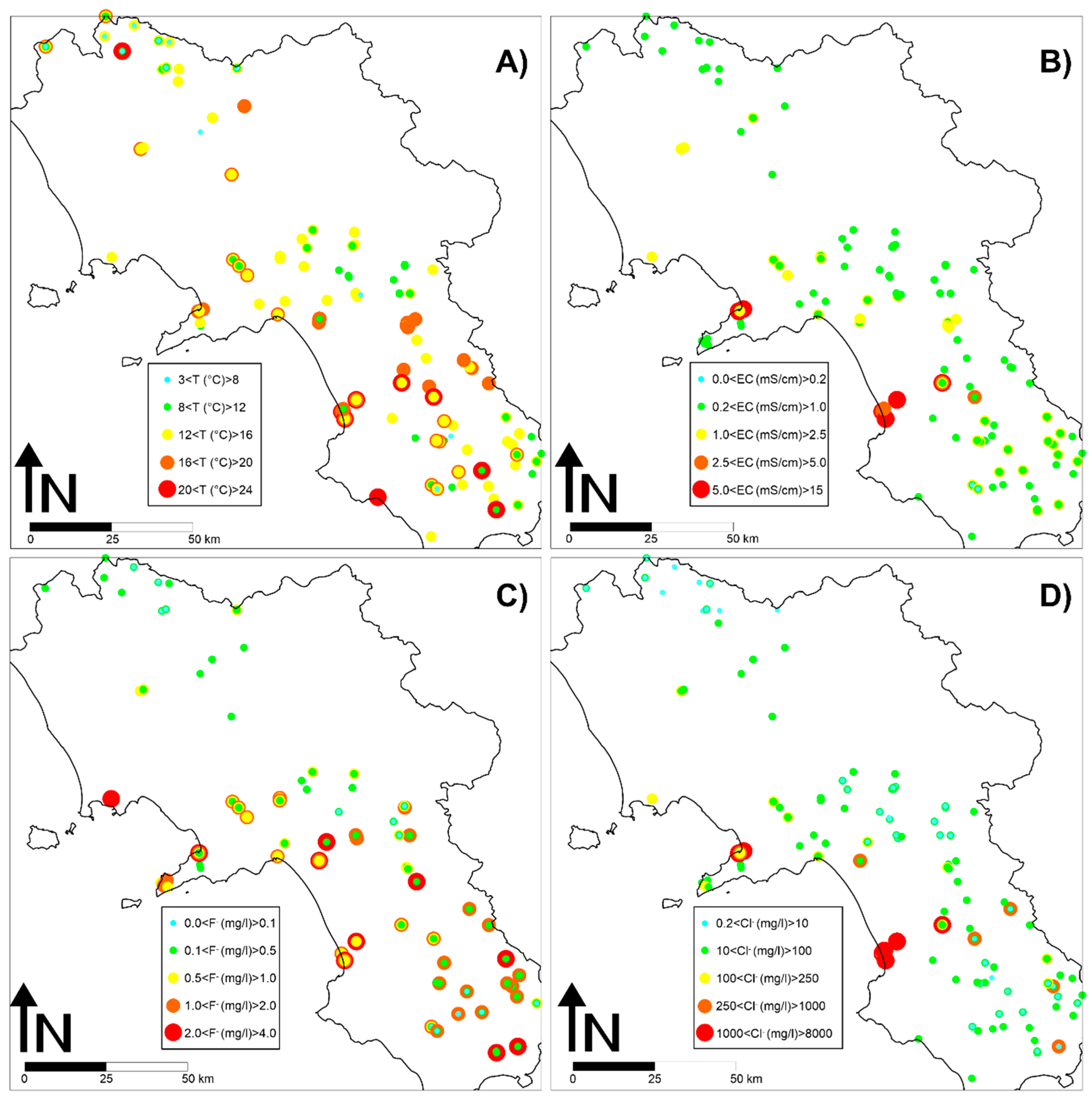
Figure 3 shows the spatial maps of all the observed spring temperatures, EC values, F− and Cl− concentrations in the study area during the period 2002–2017. Values for pH are not plotted since more than 90% of samples were circumneutral or slightly alkaline, values typical of well buffered systems such as the carbonate aquifers. The few anomalous values were recorded in springs pertaining to volcanic or fault systems.
The springs with elevated temperatures (20 °C < temperatures < 24 °C) are located in areas characterized by elevated geothermal gradients induced by volcanic activity or regional faults [35,36]. Only few springs are characterized by elevated EC values (EC > 1000 µS/cm) and thus highly mineralized, all the others are in the range of oligomineral or mineral freshwaters typical for karst aquifers. It should be noted that a few springs near the coast are characterized by elevated EC and Cl− concentrations, these are the famous mineral springs of Paestum and Castellamare di Stabia. These springs are not affected by seawater intrusion, but their elevated salinity derives from the deep circulation in karst systems along faults [35,36]. Figure 3 highlights that the Cl− spatial distribution in spring water mimics the EC spatial distribution, while the F− spatial distribution in spring water mimics the springs’ temperature spatial distribution. Cl− is a well-known environmental tracer, since it is not involved in biogeochemical reactions, nor is it adsorbed on clay minerals; thus, it is usually directly related to the residence time in aquifers, with low concentrations in shallow systems and increasing concentrations with increasing residence times and flow paths [37]. So, the fact that Cl− mimics the EC in springs water (which, in turn, is a proxy of water mineralization), suggests longer flow paths with increasing Cl− concentrations [38]. On the other hand, F− is not a conservative tracer, since it usually undergoes precipitation and dissolution processes in neo-formed mineral phases like fluorite or fluorapatite. For this reason, the increase of spring water temperatures is usually related to an increase of F− concentration in water [39] when F– is present in the aquifer matrix [40]. The lithological map is shown in Figure 4, with the main faults and the maximum, minimum and average springs temperatures available from the database. It can be noticed that most of the spring outflow is from karstified limestones, which form the main aquifers of this region [41]. Additionally, the springs with highest maximum, minimum and average temperatures are aligned on the main fault system, making evident the structural control of the groundwater flow system. These springs are the ones with lowest range of temperature variability (Figure 4), since they are fed by a deep circulation system. This brief spatial description of the water parameters analysed highlights the complexity of the aquifer systems of the Campania region. Additionally, there are various geothermal heat sources that contribute to the puzzle of the observed spring water temperatures, with respect to climate induced temperature variations. In addition, springs elevation should also be considered for a comprehensive analysis of water temperature variation, as discussed in the next section.
3.3. Vertical Spring Water Temperatures and EC Variations
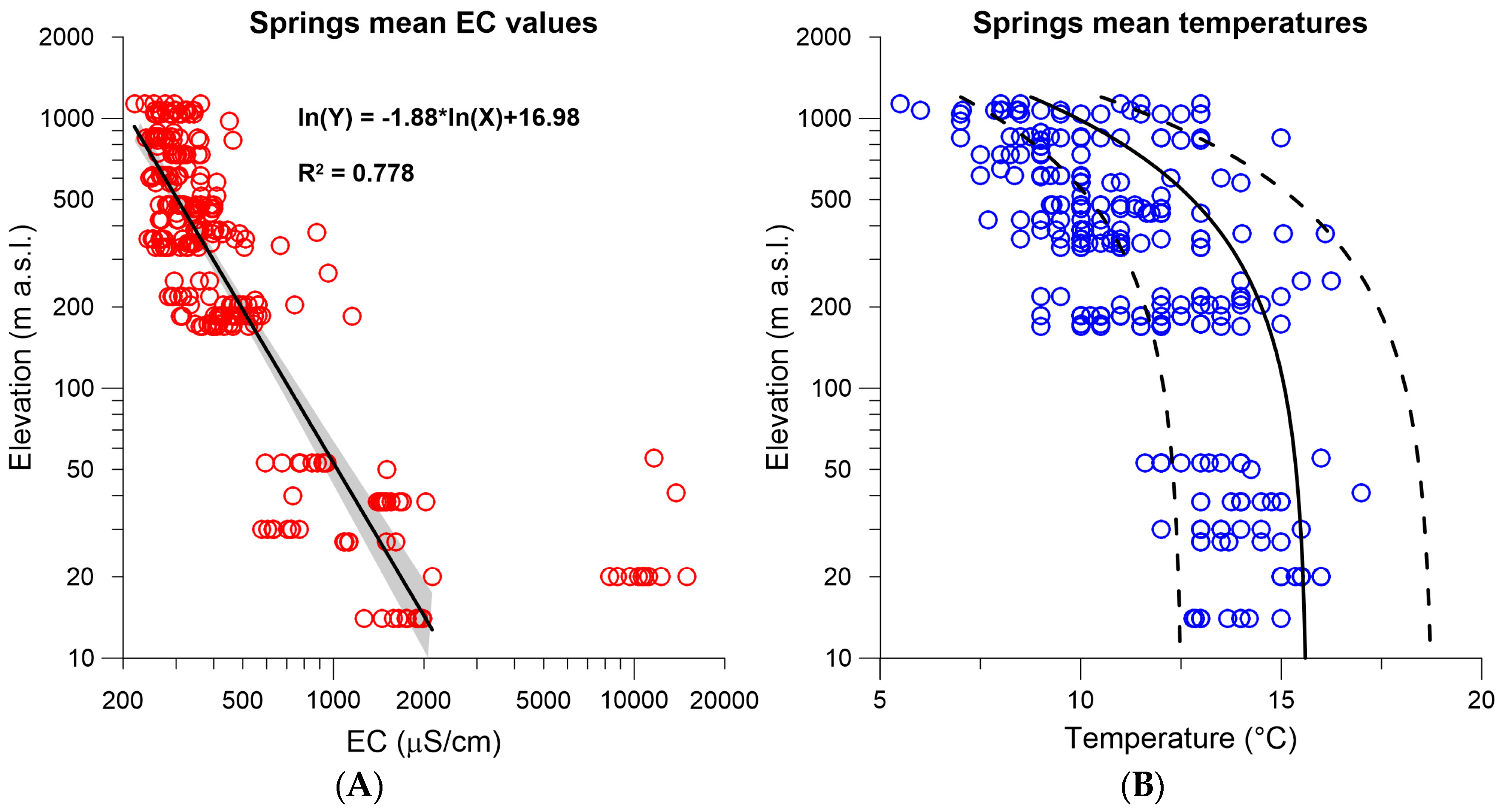
Figure 5 shows that the mean EC variation with altitude in the monitored springs is reasonably well represented by a power law, if we exclude the most mineralized springs (Paestum and Castellamare di Stabia), which cluster together around the EC value of 10,000 µS/cm.
This confirms that, at the regional scale, the residence times in the Campania aquifers decrease with the spring’s elevation [36], although, the large EC variability and the narrow bands of 95% confidence intervals of Figure 4 denote that, at the local scale, aquifer heterogeneities might lead to very different flow paths. Like spring water EC mean values, the spring water temperatures highlight some differences with respect to the mean air–altitude gradient of −0.64 °C/100 m calculated for the Campania region [41]. Most of the water samples fall within the confidence interval set at ±20% respective to the mean air–altitude gradient to account for climatic variability, which is similar to a recent study in the upper Volturno valley [36], although in that study, higher than usual water temperatures were linked with active faults. In this study a large sample group falls below the expected limits, and just a few samples are above the expected limits. The reason for this behaviour is probably due to concentrated recharge from snow melting during springtime [42], which can promote water temperature decrease especially in springs located at higher altitudes.
3.4. Spring Water Temperatures and Water Quality Temporal Trends
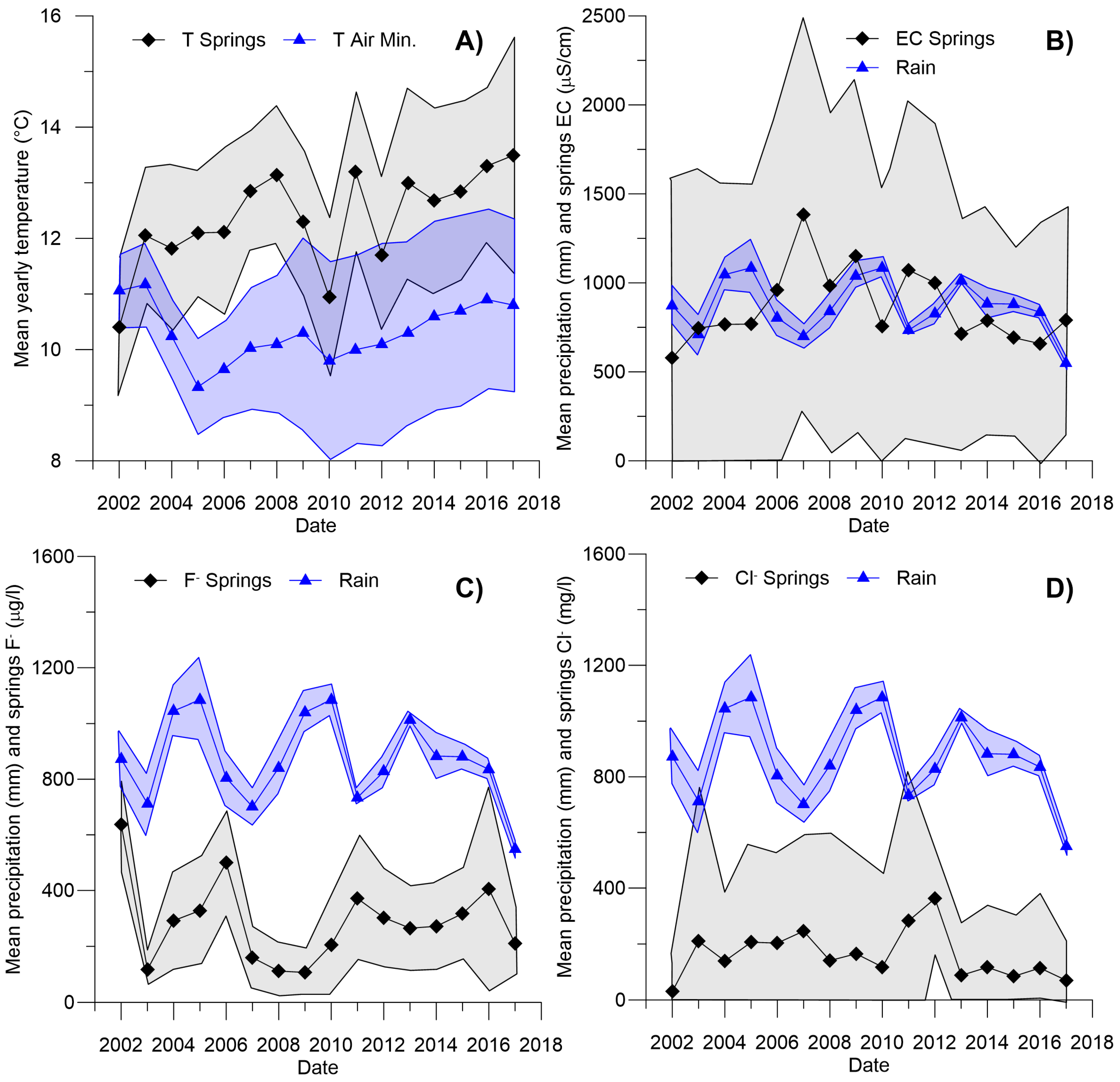
An indisputable increase of spring water temperatures is shown by the annual mean spring temperatures plot of Figure 6, with an increasing trend of approximately +0.12 °C/y. Nevertheless, this linear relationship is characterized by a low R2, with a value of 0.40. The annual increment is compatible with the one found for the minimum atmospheric temperatures of the Campania region in the same period. Despite the online database containing a very large number of groundwater temperatures and water quality data, it was decided not to use the groundwater dataset, since no information was available on the depth of the observed data. In fact, the observed groundwater temperatures could be biased by multiple factors, like the long screens of the investigated wells that could cause artificial mixing of different waters, or measurement methods that could be influenced by atmospheric temperatures [43].
Only a small area of the Campania region was previously studied for possible connections between climate change and groundwater temperatures response [21], but in that area, the monitoring well depths were known with relatively good accuracy. It should be stressed that a very similar groundwater temperature trend of +0.13 °C/y was found in that study, respective to the springs water temperatures trend found here. In addition to spring water temperature increases, Figure 5 shows other remarkable trends associated with spring water quality; for example, the EC values tend to decrease in years characterized by high precipitation and to increase in dry years. Despite this general rule, the standard deviations of EC values at the regional scale are extremely elevated, due to the presence of hydrothermal systems near volcanic districts and deep circulation along faults, as outlined in Section 3.2, and due to orographic effects, as outlined in Section 3.3. Much lower standard deviation values were shown by Cl− concentrations in springs water, but the same trend was seen as for the EC values. Even lower standard deviation values were shown by the F– concentrations in spring water, although a less clear inverse relationship with the precipitations is deducible. In fact, F− concentrations in spring water seem to be retarded respective to the precipitation, but the available data were not sufficient to prove this hypothesis. In general, the dataset on spring water EC and Cl− concentrations suggests that a decrease in precipitation leads to increased mineralization, and that this could be due to a higher proportion of storage water respective to run-off water in dry years. Given that the springs are characterized by very different residence times [30,35,41], it is unlikely that recharge waters with increased water temperatures have already reached all the springs. Thus, a possible explanation is that the positive shift of minimum atmospheric temperatures is driving the springs water temperature increase by heat exchange via near surface thermal diffusion. Finally, it must be stressed that the analysed water quality parameters (pH not shown) did not increase with time as temperatures did over the monitored period, but showed much more complex behaviour, linked with the precipitation variability over the analysed period of time.
3.5. Linear and Multivariate Statistical Analysis
The Pearson coefficient between yearly atmospheric temperatures, precipitations and spring water quality parameters was not significant, except for the EC values and Cl− concentrations with a value of 0.65 at p < 0.05. As explained in Section 3.2, the positive relationship between EC values and Cl− concentrations is due to the residence time of groundwater with increasing flow paths. The R-Type FA was applied to identify possible correlations between physical and chemical parameters of the Campania springs. The analysis was performed with 16 variables: T Min, T Max, T Ave, EC Min, EC Max, EC Ave, pH Min, pH Max, pH Ave, Cl− Min, Cl− Max, Cl− Ave, F− Min, F− Max, F− Ave and spring elevation (Elevation). Elevation values were extracted from a digital elevation model (DEM), while minimum, maximum and average values of all variables were calculated for the whole monitored period. From the FA analysis, four factors emerged over the 95% confidence interval (Table 2), with a KMO higher than 0.5 (0.76). These four factors explain 83% of the total variance. The first factor explains 33% of the total variance, and shows high positive correlations between EC values and Cl− concentrations. Factor 2 explains 20% of variance and is linked to the altitude zonation. A negative correlation was found between T Min and Elevation; therefore, a decrease of elevation in relation to the increase of minimum and average water temperature, which seems also connected to the increase of F− content in spring waters (F− Min). The spring temperature seems to be mainly influenced by vertical zonation, because there are no statistically significant differences in temperature (T Min, T Max, T Ave) between springs located in different geological formations. This assumption is also confirmed by Table 3, which shows the temperature variations for the three main hydrogeological systems: limestones, flysches and alluvial deposits. The third factor has a moderate correlation between T Max and F− Max, explaining 18% of the variance. It enforces the assumption that the F– concentration in springs water increases directly with the increase of temperature. Finally, the last factor (12% of variance) involves only pH values (pH Min, pH Max, pH Av) and seems to be independent from other parameters, or at least extremely weakly correlated, as stated in Section 3.2.
Additionally, the ANOVA test performed on the three main hydrogeological systems highlighted that there is no statistical difference between the three populations of data for T Min, T Max and T Ave. This implies that the spring temperature variations are more likely linked to the air temperature at the Campania region scale than to the lithological formations to which they pertain.
4. Conclusions
This study has shown a clear correlation between the increase of yearly average minimum atmospheric temperatures and the concurrent increase of the yearly average spring water temperatures of the Campania region, located in Southern Italy. The investigated area has experienced an increase of spring water temperatures of approximately 2.0 °C in the period from 2002 to 2017. The positive shift of minimum atmospheric temperatures is probably linked to the spring water temperature increase by near surface thermal exchange, and not by increased water temperatures of recharge waters. This is because a concomitant increase of water parameters like EC, pH, Cl− and F− was not recorded during the monitoring period. These water quality parameters are more probably linked to the precipitation trend and other local factors like spring altitude, different residence times and presence of geothermal heat fluxes. Despite the good correlation found between minimum atmospheric temperatures and springs water temperatures, this assessment study should be further implemented to unravel possible long-term effects of this phenomenon, which could, in the long run, affect spring water quality.
Author Contributions
Conceptualization, M.M.; Data curation, M.M.; Formal analysis, G.B. and N.C.; Funding acquisition, M.M.; Methodology, N.C.; Software, G.B.; Writing—original draft, N.C.; Writing—review & editing, M.M.
Funding
This research was funded by FFABR 2017.
Conflicts of Interest
The authors declare no conflict of interest. The founding sponsors had no role in the design of the study; in the collection, analyses, or interpretation of data; in the writing of the manuscript, and in the decision to publish the results.
References
- Cramer, W.; Guiot, J.; Fader, M.; Garrabou, J.; Gattuso, J.-P.; Iglesias, A.; Lange, M.A.; Lionello, P.; Llasat, M.C.; Paz, S.; et al. Climate change and interconnected risks to sustainable development in the Mediterranean. Nat. Clim. Chang. 2018, 8, 972–980. [Google Scholar] [CrossRef]
- Candela, L.; Elorza, F.J.; Jiménez-Martínez, J.; von Igel, W. Global change and agricultural management options for groundwater sustainability. Comput. Electron. Agric. 2012, 86, 120–130. [Google Scholar] [CrossRef]
- Chaouche, K.; Neppel, L.; Dieulin, C.; Pujol, N.; Ladouche, B.; Martin, E.; Salas, D.; Caballero, Y. Analyses of precipitation, temperature and evapotranspiration in a French Mediterranean region in the context of climate change. C. R. Geosci. 2010, 342, 234–243. [Google Scholar] [CrossRef]
- Molina-Navarro, E.; Trolle, D.; Martínez-Pérez, S.; Sastre-Merlín, A.; Jepsen, E. Hydrological and water quality impact assessment of a Mediterranean limno-reservoir under climate change and land use change scenarios. J. Hydrol. 2014, 509, 354–366. [Google Scholar] [CrossRef]
- Dai, A. Increasing drought under global warming in observations and models. Nat. Clim. Chang. 2013, 3, 52–58. [Google Scholar] [CrossRef]
- Lionello, P. The Climate of the Mediterranean Region: From the Past to the Future; Elsevier: New York, NY, USA, 2012; 592p. [Google Scholar]
- Bates, B.; Kundzewicz, Z.W.; Wu, S.; Palutikof, J.P. Climate Change and Water, Intergovernmental Panel on Climate Change Secretariat; IPCC Secretariat: Geneva, Switzerland, 2008; 210p. [Google Scholar]
- Giorgi, F.; Im, E.-S.; Coppola, E.; Diffenbaugh, N.S.; Gao, X.J.; Mariotti, L.; Shi, Y. Higher hydroclimatic intensity with global warming. J. Clim. 2011, 24, 5309–5324. [Google Scholar] [CrossRef]
- Hirabayashi, Y.; Mahendran, R.; Koirala, S.; Konoshima, L.; Yamazaki, D.; Watanabe, S.; Kim, H.; Kanae, S. Global flood risk under climate change. Nat. Clim. Chang. 2013, 3, 816–821. [Google Scholar] [CrossRef]
- Garner, G.; Hannah, D.M.; Watts, G. Climate change and water in the UK: Recent scientific evidence for past and future change. Prog. Phys. Geogr. 2017, 41, 1–17. [Google Scholar] [CrossRef]
- Stuart, M.E.; Gooddy, D.C.; Bloomfield, J.P.; Williams, A.T. A review of the impact of climate change on future nitrate concentrations in groundwater of the UK. Sci. Total Environ. 2011, 409, 2859–2873. [Google Scholar] [CrossRef] [Green Version]
- Taylor, R.G.; Scanlon, B.; Döll, P.; Rodell, M.; Van Beek, R.; Wada, Y.; Longuevergne, L.; Leblanc, M.; Famiglietti, J.S.; Edmunds, M.; et al. Ground water and climate change. Nat. Clim. Chang. 2013, 3, 322–329. [Google Scholar] [CrossRef]
- Green, T.R.; Taniguchi, M.; Kooi, H.; Gurdak, J.J.; Allen, D.M.; Hiscock, K.M.; Treide, H.; Aureli, A. Beneath the surface of global change: Impacts of climate change on groundwater. J. Hydrol. 2011, 405, 532–560. [Google Scholar] [CrossRef]
- Jyrkama, M.I.; Sykes, J.F. The impact of climate change on spatially varying groundwater recharge in the grand river watershed (Ontario). J. Hydrol. 2007, 338, 237–250. [Google Scholar] [CrossRef]
- Hannah, D.M.; Garner, G. River water temperature in the United Kingdom: Changes over the 20th century and possible changes over the 21st century. Prog. Phys. Geogr. 2015, 39, 68–92. [Google Scholar] [CrossRef] [Green Version]
- Selbig, W.R. Simulating the effect of climate change on stream temperature in the Trout LakeWatershed, Wisconsin. Sci. Total Environ. 2015, 521–522, 11–18. [Google Scholar] [CrossRef] [PubMed]
- Wenger, S.J.; Isaak, D.J.; Luce, C.H.; Neville, H.M.; Fausch, K.D.; Dunham, J.B.; Dauwalter, D.C.; Young, M.K.; Elsner, M.M.; Rieman, B.E.; et al. Flow regime, temperature, and biotic interactions drive differential declines of trout species under climate change. Proc. Natl. Acad. Sci. USA 2011, 108, 14175–14180. [Google Scholar] [CrossRef] [PubMed]
- Houben, G.J.; Koeniger, P.; Sultenfuß, J. Freshwater lenses as archive of climate, groundwater recharge, and hydrochemical evolution: Insights from depth-specific water isotope analysis and age determination on the island of Langeoog, Germany. Water Resour. Res. 2014, 50, 8227–8239. [Google Scholar] [CrossRef] [Green Version]
- Menberg, K.; Blum, P.; Kurylyk, B.L.; Bayer, P. Observed groundwater temperature response to recent climate change. Hydrol. Earth Syst. Sci. 2014, 18, 4453–4466. [Google Scholar] [CrossRef] [Green Version]
- Kurylyk, B.L.; MacQuarrie, K.T.B.; Voss, C.L. Climate change impacts on the temperature and magnitude of groundwater discharge from shallow unconfined aquifers. Water Resour. Res. 2014, 50, 3253–3274. [Google Scholar] [CrossRef]
- Mastrocicco, M.; Busico, G.; Colombani, N. Groundwater Temperature Trend as a Proxy for Climate Variability. Proceedings 2018, 2, 630. [Google Scholar] [CrossRef]
- Casciello, E.; Cesarano, M.; Pappone, G. Extensional detachment faulting on the Tyrrhenian margin of the southern Apennines contractional belt (Italy). J. Geol. Soc. 2006, 163, 617–629. [Google Scholar] [CrossRef]
- Ducci, D.; Tranfaglia, G. The Effect of Climate Change on the Hydrogeological Resources in Campania Region (Italy). In Groundwater and Climatic Changes; Dragoni, W., Ed.; Geological Society of London: London, UK, 2008; Volume 288, pp. 25–38. [Google Scholar] [CrossRef]
- Busico, G.; Kazakis, N.; Colombani, N.; Mastrocicco, M.; Voudouris, K.; Tedesco, D. A modified SINTACS method for groundwater vulnerability and pollution risk assessment in highly anthropized regions based on NO3− and SO42− concentrations. Sci. Total Environ. 2017, 609, 1512–1523. [Google Scholar] [CrossRef] [PubMed]
- Ducci, D.; Della Morte, R.; Mottola, A.; Onorati, G.; Pugliano, G. Nitrate trends in groundwater of the Campania region (southern Italy). Environ. Sci. Pollut. Res. 2017, 26, 1–12. [Google Scholar] [CrossRef] [PubMed]
- Minolfi, G.; Albanese, S.; Lima, A.; Tarvainen, T.; Fortelli, A.; De Vivo, B. A regional approach to the environmental risk assessment—Human health risk assessment case study in the Campania region. J. Geochem. Explor. 2016, 184, 400–416. [Google Scholar] [CrossRef]
- ARPA Campania. Available online: http://www.arpacampania.it/web/guest/365 (accessed on 23 December 2018).
- Regione Campania. Available online: http://www.agricoltura.regione.campania.it/meteo/agrometeo.htm (accessed on 23 December 2018).
- Ministero Delle Politiche Agricole Alimentari, Forestali e del Turismo. Available online: https://www.politicheagricole.it/flex/FixedPages/Common/miepfy700_provincie.php/L/IT?name=00092&%20name1=15 (accessed on 23 December 2018).
- De Vita, P.; Allocca, V.; Manna, F.; Fabbrocino, S. Coupled decadal variability of the North Atlantic Oscillation, regional rainfall and karst spring discharges in the Campania region (southern Italy). Hydrol. Earth Syst. Sci. 2012, 16, 1389–1399. [Google Scholar] [CrossRef] [Green Version]
- Busico, G.; Cuoco, E.; Kazakis, N.; Colombani, N.; Mastrocicco, M.; Tedesco, D.; Voudouris, K. Multivariate statistical analysis to characterize/discriminate between anthropogenic and geogenic trace elements occurrence in the Campania plain, southern Italy. Environ. Pollut. 2018, 234, 260–269. [Google Scholar] [CrossRef] [PubMed]
- Żelazny, M.; Rajwa-Kuligiewicz, A.; Bojarczuk, A.; Pęksa, Ł. Water temperature fluctuation patterns in surface waters of the Tatra Mts., Poland. J. Hydrol. 2018, 564, 824–835. [Google Scholar] [CrossRef]
- Kaiser, H.F. The varimax criterion for analytic rotation in factor analysis. Psychometrika 1958, 23, 187–200. [Google Scholar] [CrossRef]
- Toreti, A.; Desiato, F.; Fioravanti, G.; Perconti, W. Seasonal temperatures over Italy and their relationship with low-frequency atmospheric circulation patterns. Clim. Chang. 2010, 99, 211–227. [Google Scholar] [CrossRef]
- Duchi, V.; Minissale, A.; Vaselli, O.; Ancillotti, M. Hydrogeochemistry of the Campania region in southern Italy. J. Volcanol. Geotherm. Res. 1995, 67, 313–328. [Google Scholar] [CrossRef]
- Cuoco, E.; Colombani, N.; Darrah, T.H.; Mastrocicco, M.; Tedesco, D. Geolithological and anthropogenic controls on the hydrochemistry of the Volturno river (Southern Italy). Hydrol. Process. 2017, 31, 627–638. [Google Scholar] [CrossRef]
- Scanlon, B.R.; Keese, K.E.; Flint, A.L.; Flint, L.E.; Gaye, C.B.; Edmunds, W.M.; Simmers, I. Global synthesis of groundwater recharge in semiarid and arid regions. Hydrol. Process. 2006, 20, 3335–3370. [Google Scholar] [CrossRef]
- Ettayfi, N.; Bouchaou, L.; Michelot, J.L.; Tagma, T.; Warner, N.; Boutaleb, S.; Massault, M.; Lgourna, Z.; Vengosh, A. Geochemical and isotopic (oxygen, hydrogen, carbon, strontium) constraints for the origin, salinity, and residence time of groundwater from a carbonate aquifer in the Western Anti-Atlas Mountains, Morocco. J. Hydrol. 2012, 438, 97–111. [Google Scholar] [CrossRef]
- Valenzuela-Vasquez, L.; Ramirez-Hernandez, J.; Reyes-Lopez, J.; Sol-Uribe, A.; Lazaro-Mancilla, O. The origin of fluoride in groundwater supply to Hermosillo City, Sonora, Mexico. Environ. Geol. 2006, 51, 17–27. [Google Scholar] [CrossRef]
- Rango, T.; Colombani, N.; Mastrocicco, M.; Bianchini, G.; Beccaluva, L. Column elution experiments on volcanic ash: Geochemical implications for the main Ethiopian rift waters. Water Air Soil Pollut. 2010, 208, 221–233. [Google Scholar] [CrossRef]
- Allocca, V.; Manna, F.; De Vita, P. Estimating annual groundwater recharge coefficient for karst aquifers of the southern Apennines (Italy). Hydrol. Earth Syst. Sci. 2014, 18, 803–817. [Google Scholar] [CrossRef] [Green Version]
- Fiorillo, F.; Esposito, L.; Guadagno, F.M. Analyses and forecast of water resources in an ultra-centenarian spring discharge series from Serino (Southern Italy). J. Hydrol. 2007, 336, 125–138. [Google Scholar] [CrossRef]
- Colombani, N.; Giambastiani, B.M.S.; Mastrocicco, M. Use of shallow groundwater temperature profiles to infer climate and land use change: Interpretation and measurement challenges. Hydrol. Process. 2016, 30, 2512–2524. [Google Scholar] [CrossRef]
Figure 1.
Hydrogeological map, with the location of the meteorological stations, the main faults and the monitored springs.
Figure 1.
Hydrogeological map, with the location of the meteorological stations, the main faults and the monitored springs.

Figure 2.
(A) Annual mean, maximum and minimum air temperatures recorded in the study area from 2002 to 2017 and their standard deviations, plotted as upper and lower lines. (B) Annual mean precipitations recorded in the study area from 2002 to 2017 and their standard deviations, plotted as upper and lower lines. (C) Mean annual maximum and minimum air temperature indexes (MATI) and (D) mean annual precipitation index (MAPI) for the Campania region.

Figure 3.
(A) Map of all the available spring water temperatures. (B) Map of all the available spring water electrical conductivity (EC) values. (C) Map of all the available spring water F− concentrations. (D) Map of all the available spring water Cl− concentrations.
Figure 3.
(A) Map of all the available spring water temperatures. (B) Map of all the available spring water electrical conductivity (EC) values. (C) Map of all the available spring water F− concentrations. (D) Map of all the available spring water Cl− concentrations.

Figure 4.
(A) Average values of maximum spring water temperatures. (B) Average values of minimum spring water temperatures. (C) Average values of mean spring water temperatures. The geological formations are in conjunction with the main fault system.
Figure 4.
(A) Average values of maximum spring water temperatures. (B) Average values of minimum spring water temperatures. (C) Average values of mean spring water temperatures. The geological formations are in conjunction with the main fault system.

Figure 5.
(A): altitude versus springs EC mean values during the monitoring period (2002–2017); the black line represents the EC–altitude power–law relationship found, excluding the highly mineralized springs (EC > 5000 µS/cm), and the grey shaded area shows the 95% confidence intervals. (B): altitude versus springs mean temperatures during the monitoring period (2002–2017); the black curve represents the temperature–altitude gradient [41], and the dashed curves a temperature variability of ±20%.

Figure 6.
(A) Annual average spring water temperatures recorded from 2002 to 2017 (black diamonds), compared with the average minimum air temperatures (blue triangles) and their standard deviations (shaded areas). (B) Annual average spring water EC (black diamonds), compared with the mean precipitations (blue triangles) and their standard deviations (shaded areas). (C) Annual average spring water F– concentration (black diamonds), compared with the mean precipitation (blue triangles) and their standard deviations (shaded areas). (D) Annual average spring water Cl– concentration (black diamonds), compared with the mean precipitations (blue triangles) and their standard deviations (shaded areas).


Table 1.
Summary of the spring water physiochemical parameters database. N° refers to the number of observations available for the selected parameter.
Table 1.
Summary of the spring water physiochemical parameters database. N° refers to the number of observations available for the selected parameter.
| Year | Temperature (°C) | EC (µS/cm) | pH (-) | Cl− (mg/L) | F− (µg/L) | ||||||||||
|---|---|---|---|---|---|---|---|---|---|---|---|---|---|---|---|
| N° | Max | Min | N° | Max | Min | N° | Max | Min | N° | Max | Min | N° | Max | Min | |
| 2002 | 36 | 15.1 | 5.2 | 36 | 2130 | 287 | 26 | 8.0 | 6.5 | 36 | 219 | 5.1 | 17 | 3200 | 0 |
| 2003 | 106 | 18.0 | 7.1 | 107 | 13,760 | 200 | 92 | 8.1 | 6.3 | 107 | 8432 | 4.5 | 15 | 425 | 0 |
| 2004 | 123 | 21.0 | 5.1 | 123 | 13,050 | 45 | 38 | 8.0 | 6.4 | 122 | 3190 | 3.7 | 33 | 1100 | 50 |
| 2005 | 111 | 18.1 | 6.0 | 111 | 12,500 | 40 | 23 | 8.7 | 6.0 | 111 | 4960 | 3.0 | 23 | 1600 | 8 |
| 2006 | 92 | 19.0 | 4.2 | 96 | 13,060 | 39 | 28 | 8.0 | 6.5 | 96 | 3650 | 5.0 | 6 | 1020 | 100 |
| 2007 | 90 | 18.0 | 8.1 | 89 | 11,390 | 253 | 25 | 7.6 | 6.3 | 89 | 3545 | 2.8 | 13 | 700 | 0 |
| 2008 | 59 | 18.1 | 6.0 | 60 | 15,000 | 258 | 51 | 8.4 | 6.5 | 60 | 7090 | 3.6 | 15 | 690 | 100 |
| 2009 | 129 | 24.0 | 5.0 | 128 | 12,610 | 255 | 117 | 9.6 | 6.1 | 128 | 5317 | 1.5 | 126 | 1800 | 30 |
| 2010 | 89 | 20.0 | 5.1 | 90 | 10,900 | 251 | 90 | 9.9 | 6.2 | 90 | 4431 | 1.8 | 70 | 458 | 25 |
| 2011 | 74 | 21.1 | 8.1 | 74 | 9270 | 238 | 73 | 8.2 | 6.0 | 74 | 7512 | 16.5 | 74 | 1050 | 550 |
| 2012 | 123 | 19.2 | 4.3 | 143 | 10,810 | 217 | 143 | 8.8 | 5.9 | 142 | 2917 | 3.2 | 71 | 1084 | 60 |
| 2013 | 94 | 22.1 | 7.8 | 157 | 8810 | 30 | 151 | 8.7 | 6.2 | 154 | 2769 | 2.6 | 157 | 1161 | 15 |
| 2014 | 149 | 22.0 | 5.4 | 196 | 8730 | 62 | 192 | 8.8 | 6.4 | 192 | 2962 | 2.2 | 192 | 3289 | 0 |
| 2015 | 134 | 24.6 | 4.4 | 172 | 8073 | 43 | 172 | 9.0 | 5.7 | 171 | 3525 | 4.0 | 170 | 1900 | 28 |
| 2016 | 127 | 24.5 | 6.5 | 155 | 9080 | 60 | 150 | 8.6 | 6.3 | 151 | 4298 | 2.1 | 151 | 8068 | 8 |
| 2017 | 101 | 23.2 | 5.0 | 101 | 9240 | 46 | 101 | 8.4 | 6.8 | 101 | 2192 | 3.0 | 101 | 1560 | 8 |
Table 2.
Factor score for the applied factor analysis (FA).
| Parameter | Factor I | Factor II | Factor III | Factor IV |
|---|---|---|---|---|
| Elevation | −0.109 | −0.760 | −0.205 | 0.166 |
| T Min | 0.308 | 0.703 | 0.221 | −0.125 |
| T Max | 0.095 | 0.081 | 0.866 | −0.055 |
| T Ave | 0.281 | 0.642 | 0.590 | −0.144 |
| EC Min | 0.879 | 0.217 | −0.151 | −0.280 |
| EC Max | 0.841 | 0.229 | 0.404 | −0.075 |
| EC Ave | 0.915 | 0.264 | 0.206 | −0.157 |
| pH Min | −0.048 | −0.062 | −0.636 | 0.604 |
| pH Max | −0.273 | −0.266 | −0.039 | 0.810 |
| pH Ave | −0.245 | −0.253 | −0.430 | 0.786 |
| Cl− Min | 0.883 | 0.111 | −0.150 | −0.223 |
| Cl− Max | 0.908 | 0.224 | 0.283 | −0.028 |
| Cl− Ave | 0.943 | 0.201 | 0.172 | −0.087 |
| F− Min | 0.229 | 0.817 | −0.052 | −0.136 |
| F− Max | 0.055 | 0.337 | 0.669 | −0.212 |
| F− Ave | 0.293 | 0.662 | 0.543 | −0.192 |
Table 3.
Spring temperature variations for the three main hydrogeological systems: limestones, flysches and alluvial deposits.
Table 3.
Spring temperature variations for the three main hydrogeological systems: limestones, flysches and alluvial deposits.
| Alluvial Sediments | |||||
| T Min | T Max | T Ave | |||
| Min | Max | Min | Max | Min | Max |
| 6 | 12.6 | 12 | 20 | 9.7 | 15.4 |
| Limestones | |||||
| T Min | T Max | T Ave | |||
| Min | Max | Min | Max | Min | Max |
| 5 | 14 | 10 | 23 | 8.5 | 15.4 |
| Flysches | |||||
| T Min | T Max | T Ave | |||
| Min | Max | Min | Max | Min | Max |
| 6 | 11 | 10 | 21 | 9 | 15.4 |
© 2019 by the authors. Licensee MDPI, Basel, Switzerland. This article is an open access article distributed under the terms and conditions of the Creative Commons Attribution (CC BY) license (http://creativecommons.org/licenses/by/4.0/).
Share and Cite
MDPI and ACS Style
Mastrocicco, M.; Busico, G.; Colombani, N. Deciphering Interannual Temperature Variations in Springs of the Campania Region (Italy). Water 2019, 11, 288. https://doi.org/10.3390/w11020288
AMA Style
Mastrocicco M, Busico G, Colombani N. Deciphering Interannual Temperature Variations in Springs of the Campania Region (Italy). Water. 2019; 11(2):288. https://doi.org/10.3390/w11020288
Chicago/Turabian StyleMastrocicco, Micòl, Gianluigi Busico, and Nicolò Colombani. 2019. "Deciphering Interannual Temperature Variations in Springs of the Campania Region (Italy)" Water 11, no. 2: 288. https://doi.org/10.3390/w11020288
Note that from the first issue of 2016, this journal uses article numbers instead of page numbers. See further details here.