Effects of Different Spatial Configuration Units for the Spatial Optimization of Watershed Best Management Practice Scenarios


1
State Key Laboratory of Resources and Environmental Information System, Institute of Geographic Sciences and Natural Resources Research, CAS, Beijing 100101, China
2
University of Chinese Academy of Sciences, Beijing 100049, China
3
Jiangsu Center for Collaborative Innovation in Geographical Information Resource Development and Application, Nanjing 210023, China
4
Key Laboratory of Virtual Geographic Environment (Nanjing Normal University), Ministry of Education, Nanjing 210023, China
5
Department of Geography, University of Wisconsin-Madison, Madison, WI 53706, USA
6
Smart City Research Center, Hangzhou Dianzi University, Hangzhou 310012, China
*
Author to whom correspondence should be addressed.
Water 2019, 11(2), 262; https://doi.org/10.3390/w11020262
Submission received: 22 December 2018
/
Revised: 27 January 2019
/
Accepted: 31 January 2019
/
Published: 2 February 2019
(This article belongs to the Special Issue Impacts of Landscape Change on Water Resources)
Abstract
:Different spatial configurations (or scenarios) of multiple best management practices (BMPs) at the watershed scale may have significantly different environmental effectiveness, economic efficiency, and practicality for integrated watershed management. Several types of spatial configuration units, which have resulted from the spatial discretization of a watershed at different levels and used to allocate BMPs spatially to form an individual BMP scenario, have been proposed for BMP scenarios optimization, such as the hydrologic response unit (HRU) etc. However, a comparison among the main types of spatial configuration units for BMP scenarios optimization based on the same one watershed model for an area is still lacking. This paper investigated and compared the effects of four main types of spatial configuration units for BMP scenarios optimization, i.e., HRUs, spatially explicit HRUs, hydrologically connected fields, and slope position units (i.e., landform positions at hillslope scale). The BMP scenarios optimization was conducted based on a fully distributed watershed modeling framework named the Spatially Explicit Integrated Modeling System (SEIMS) and an intelligent optimization algorithm (i.e., NSGA-II, short for Non-dominated Sorting Genetic Algorithm II). Different kinds of expert knowledge were considered during the BMP scenarios optimization, including without any knowledge used, using knowledge on suitable landuse types/slope positions of individual BMPs, knowledge of upstream–downstream relationships, and knowledge on the spatial relationships between BMPs and spatial positions along the hillslope. The results showed that the more expert knowledge considered, the better the comprehensive cost-effectiveness and practicality of the optimized BMP scenarios, and the better the optimizing efficiency. Thus, the spatial configuration units that support the representation of expert knowledge on the spatial relationships between BMPs and spatial positions (i.e., hydrologically connected fields and slope position units) are considered to be the most effective spatial configuration units for BMP scenarios optimization, especially when slope position units are adopted together with knowledge on the spatial relationships between BMPs and slope positions along a hillslope.
1. Introduction
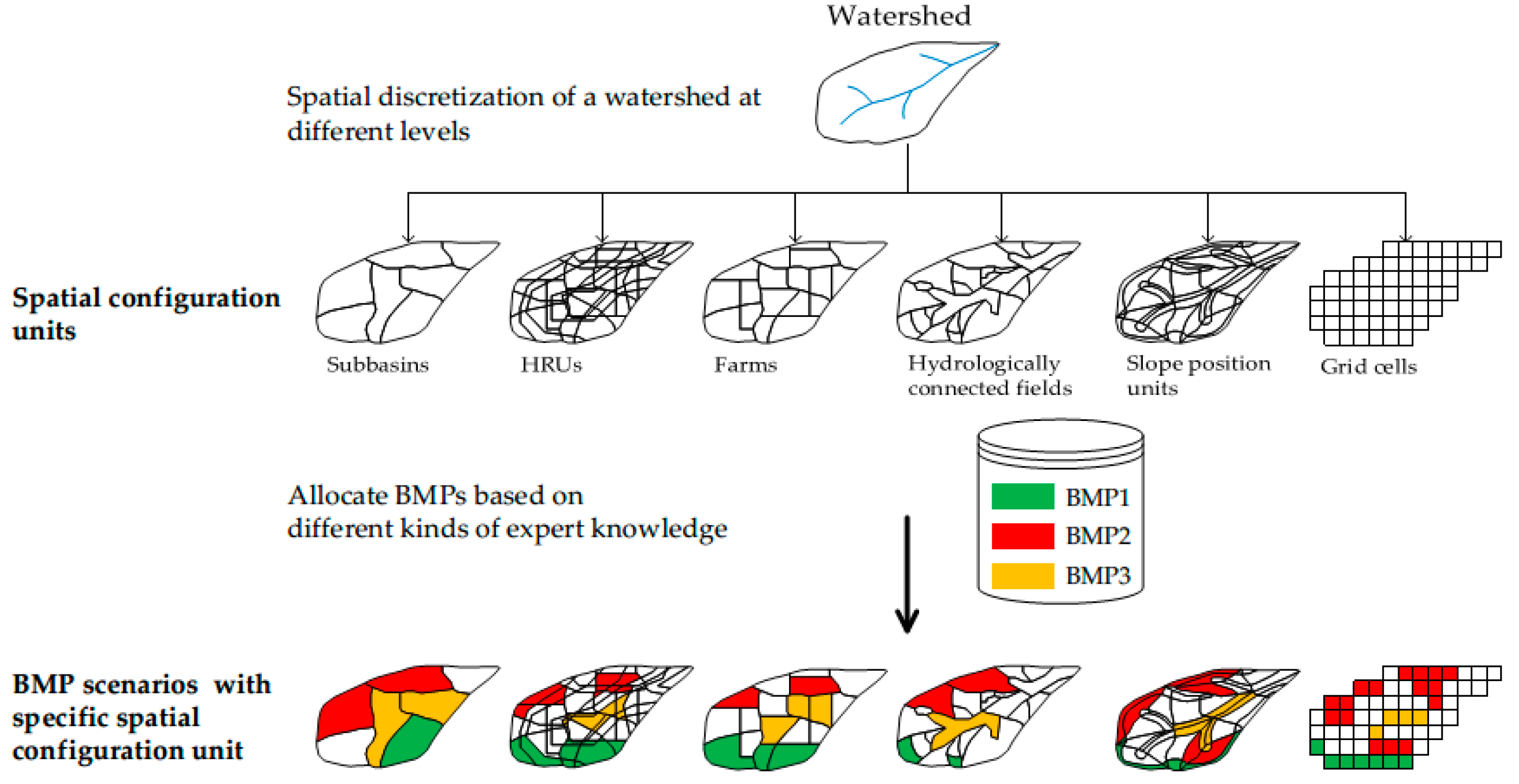
Different best management practices (or beneficial management practices, BMPs for short) scenarios (i.e., spatial configurations of multiple BMPs) at the watershed scale may have significantly different environmental effectiveness, economic efficiency, and practicality [1,2,3,4,5,6]. They are valuable for decision-making of integrated watershed management to assess the environmental effectiveness and economic efficiency of watershed BMP scenarios and then propose optimal ones. Currently, a popular approach to achieving this target is based on watershed modeling [7,8,9] coupled with intelligent optimization algorithms [2,4,5,10,11,12,13], so-called BMP scenarios optimization. To conduct the BMP scenarios optimization, each individual BMP scenario is created by automatically selecting and allocating BMPs on spatial configuration units (also called BMP configuration units hereafter), which have resulted from the spatial discretization of a watershed at one among different levels (such as subbasins, and hydrologic response units; Figure 1). When a specific type of BMP configuration unit is chosen for the BMP scenarios optimization of a watershed, normally each individual BMP configuration unit in the watershed is allowed to be configured with only one type of BMP (as the situation in this study). Then the effects of the scenario on watershed behavior are simulated by watershed models [4,13]. The simulation result is the basis of the automatic spatial optimization of BMP scenarios. Therefore, the determination of the BMP configuration units becomes the one key issue for the BMP scenarios optimization.
Currently, spatial configuration units used in BMP scenarios optimization mainly include five types with different levels, i.e., subbasins [14,15,16,17], hydrologic response units (HRUs) [12,18,19], farms [10,11], hydrologically connected fields [5], and slope position units (i.e., landform positions at hillslope scale, such as ridge, backslope, etc.) [2].
Subbasins are normally regarded as relatively closed and independent spatial configuration units which can be further delineated into different levels of spatial configuration units such as landform positions, HRUs, and gridded cells [20]. Thus, subbasins are coarse-grained units for configuring spatially explicit BMPs, and it is suitable to serve as BMP configuration units for situations in which the potential locations of BMPs are predefined within each subbasin [17]. Meanwhile, using subbasins as BMP configuration units can decrease the search space of spatial optimization more than that of the adoption of other more detailed spatial configuration units, and thus can achieve a better optimizing efficiency [15]. However, using subbasins as BMP configuration units is not available for configuring multiple spatially explicit BMPs within one subbasin while BMPs often have different effects on different spatial positions of a hillslope [2,21,22].
HRUs are delineated as hydrologic homogeneous areas according to landuse, soil, and topography (commonly presented through slope percentage) within one subbasin [23]. HRUs are extensively used for the sake of convenience, especially when the Soil and Water Assessment Tool (SWAT) [23] is applied to watershed modeling. However, an HRU is spatially discrete—it may occupy the hillslope from ridge to valley bottom—and is even spatially ambiguous when the three thresholds introduced in SWAT for delineating HRUs (i.e., the minimum percentage of the landuse area over the subbasin area, the soil area over the landuse area, and the slope class area over the soil area) are set as non-zero values [24]. Although setting these thresholds to be non-zero can reduce the count of HRUs and hence improve the computational efficiency of simulations, the inappropriate representation of the study area may introduce some levels of ambiguity in simulations. Therefore, the selected optimal BMP scenarios may not be easy to implement spatially explicitly. Similar to subbasins, HRUs are also inappropriate to serve as BMP configuration units for spatially explicit BMPs. Furthermore, the impact of BMPs of an upslope HRU on a downslope HRU cannot be represented [24], although this impact is important for incorporating the expert knowledge of spatial relationships between BMPs and spatial positions [2,5].
To improve the practicality of BMP scenarios, some studies adopted farms [10,11], or the so-called spatially explicit HRUs that are directly defined by farm boundaries [25] or landuse/landcover field maps [26], as BMP configuration units. These BMP configuration units are spatially one-to-one matched with farm or landuse/landcover fields and thus can be collectively referred to as spatially explicit HRUs [26]. Compared with spatially discrete HRUs, spatially explicit HRUs can make corresponding BMP scenarios more practical to stakeholders (such as farmers, landowners, or land managers). Meanwhile, due to the ignorance of topographic variance inside each farm or landuse/landcover field, such BMP configuration units normally have a smaller count than spatially discrete HRUs for a study area, which means higher optimizing efficiency [1,26]. However, there are still no explicitly defined upstream–downstream relationships between spatially explicit HRUs, which means that the spatial relationships between BMPs and spatial positions cannot be represented effectively [2,5].
Wu et al. [5] proposed hydrologically connected fields with upstream–downstream relationships to be BMP configuration units, which can be delineated by considering spatial topology based on flow directions and a landuse map. With hydrologically connected fields, a set of expert rules of BMP interactions based on the upstream–downstream relationships can be developed in the form of “if-then” rules, i.e., if a field has been configured with one BMP, its adjacent upstream fields should not be configured with BMP, otherwise, BMP will be randomly selected and configured on the adjacent upstream fields according to their landuse type [5]. To the best of our knowledge, the study of Wu et al. [5] is the first work on incorporating the spatial relationships between BMPs and spatial positions into BMP scenarios optimization, so that its cost-effectiveness and optimizing efficiency could be improved. However, hydrologically connected fields may be delineated across multiple landform positions or subbasins, since the hydrological relationship, considered by Wu et al. [5], is built at the watershed scale rather than the hillslope or subbasin scale. This means that hydrologically connected fields have weak spatial relationships to homogeneous functional units at the hillslope scale from the perspectives of physical geography such as geomorphic, soil, and hydrologic conditions [2]. Therefore, hydrologically connected fields also face the shortcoming that the spatially explicit BMPs cannot be represented effectively. A possible way for spatially explicit HRUs and hydrologically connected fields to overcome the above-mentioned shortcoming is to delineate them so as to be small enough patchworks of gridded cells within homogeneous functional units, or even individual gridded cells [27,28,29]. However, this approach will render the optimization based on such spatial configuration units computationally intensive or even unsolvable [27]. This makes such an approach only suitable for the spatial optimization of one single BMP within a little watershed [28,29], thus having too narrow applicability for normal watershed management which considers multiple BMPs.
More recently, Qin et al. [2] proposed slope position units [30,31] as BMP configuration units, so as to overcome the above-mentioned shortcomings of hydrologically connected fields and other BMP configuration units. Slope position units (e.g., ridge, backslope, and valley), as spatially contiguous and topographically connected units along the hillslope, are inherently related to physical watershed processes [20,30,32], and thus affect the effectiveness of BMPs [2]. Besides, the count of slope position units is comparatively limited, so as to ensure optimizing efficiency. Therefore, the spatial relationships between BMPs and slope positions along the hillslope could be explicitly and effectively considered during the spatial optimization of BMP scenarios. According to the preliminary study [2], this spatial-relationship-considered way of using slope position units as BMP configuration units is effective, efficient, and practical for BMP scenarios optimization, compared to a standard random optimization way of selecting and allocating BMPs randomly on configuration units.
Although many studies have assessed the cost-effectiveness of each individual type of above-mentioned BMP configuration units for the spatial optimization of BMP scenarios, as far as we know, a comparison among main types of BMP configuration units based on the same one watershed model for an area is still lacking. To discuss the effects of different BMP configuration units for watershed BMP scenarios optimization with regard to cost-effectiveness, optimizing efficiency, and practicality, this paper compares four types of BMP configuration units (i.e., HRUs, spatially explicit HRUs, hydrologically connected fields, and slope position units) in the spatial optimization of configuring multiple spatially explicit BMPs for mitigating soil erosion based on a spatially distributed watershed model. Subbasins are not included in this study, because subbasins are too coarse-grained to represent multiple spatially explicit BMPs.
2. Materials and Methods
2.1. Methodology
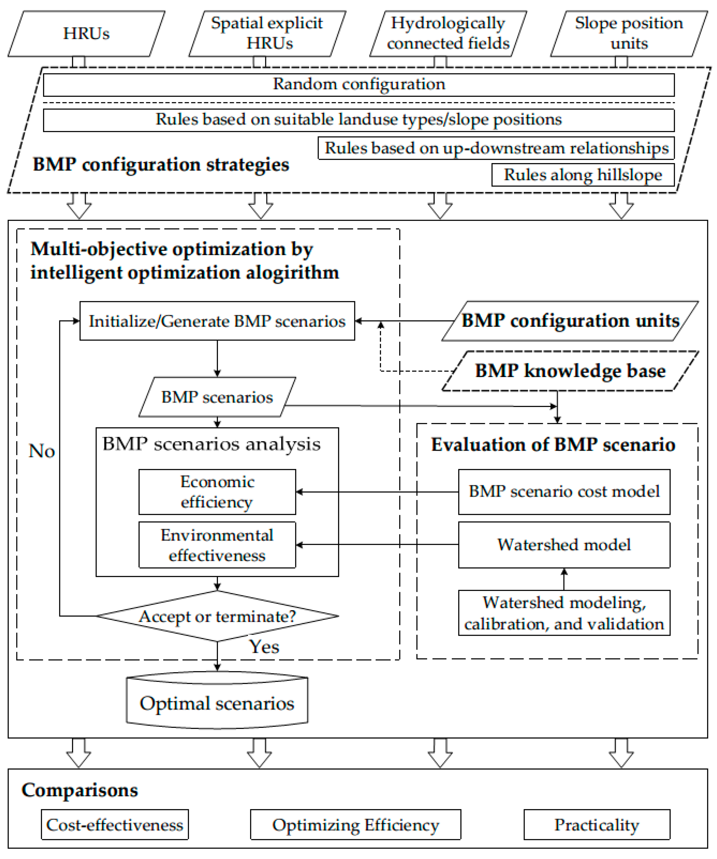
To compare the effects of these four types of BMP configuration units for watershed BMP scenarios optimization, a widely used spatial optimization framework of BMP scenarios based on watershed modeling coupled with intelligent optimization algorithms [2,10,12] was adopted in this study. As shown in Figure 2, the spatial optimization framework of watershed BMP scenarios mainly consists of four components: (1) BMP configuration units for allocating BMPs within the watershed; (2) a BMP knowledge base together with BMP configuration units as inputs to generate and evaluate BMP scenarios; (3) models for evaluating each watershed BMP scenario, including a distributed watershed model that can simulate spatial interactions between spatially explicitly distributed BMPs and effectively assess the environmental effectiveness of each BMP scenario [2,5,33], and a BMP scenario cost model for estimating the economic efficiency of each BMP scenario; (4) a multi-objective optimization component based on an intelligent optimization algorithm such as NSGA-II (Non-dominated Sorting Genetic Algorithm II) [34], which includes initializing BMP scenarios based on BMP configuration units and a BMP knowledge base, and generating new BMP scenarios or proposing optimal ones based on the evaluation results of all current BMP scenarios. These components are elaborated in four subsections (Section 2.3, Section 2.4, Section 2.5 and Section 2.6) followed by the subsection of the study area and dataset (Section 2.2).
Besides knowledge on the environmental effectiveness and cost-benefit of individual BMPs, BMP configuration knowledge (such as the suitable landuse types/slope positions for individual BMPs, and the spatial relationships between BMPs and spatial positions) is necessary for BMP scenarios optimization (Figure 2). According to the characteristics of BMP configuration units, different kinds of BMP configuration knowledge can be saved in the BMP knowledge base and applied (hereafter referred to as BMP configuration strategy) (Figure 2). For example, the simple rule of suitable landuse types/slope positions is applicable for all types of BMP configuration units, while the expert rules based on upstream–downstream relationships between BMPs can only be applied to the BMP configuration units which have upstream–downstream relationships [5], such as hydrologically connected fields and slope position units. Furthermore, the expert rules based on the spatial relationships between BMPs and slope positions along the hillslope are only applicable for slope position units [2]. Section 2.4 contains more detailed information about the BMP knowledge base and BMP configuration strategies adopted in this study.
To assess the effects of four types of BMP configuration units for watershed BMP scenarios optimization, all feasible combinations of BMP configuration units and BMP configuration strategies were investigated by the same watershed BMP scenarios optimization framework (Figure 2). The results of different BMP configuration units applied with available BMP configuration strategies are discussed from the perspectives of cost-effectiveness, optimizing efficiency, and practicality (Figure 2). The detailed experimental design is described in Section 2.7.
2.2. Study Area and Dataset
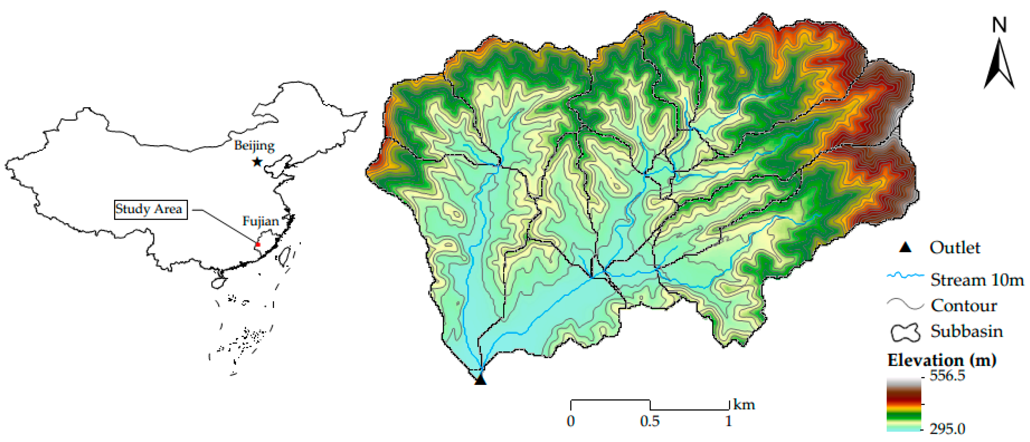
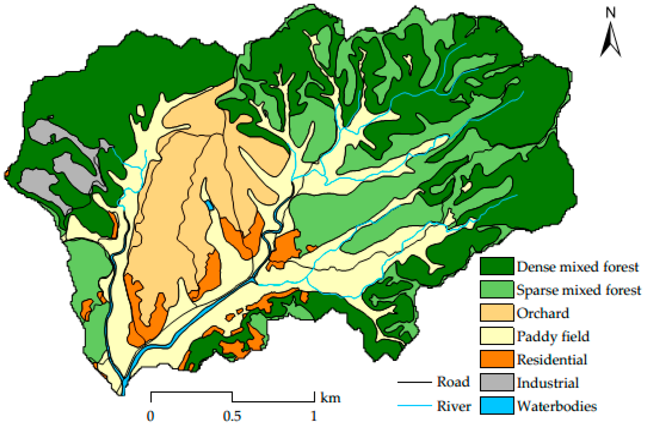
The Youwuzhen watershed (~5.39 km2), located in the typical severely eroded red-soil hilly region in southeastern China, was selected as the study area (Figure 3). Low hills with steep slopes (up to 52.9° and with an average slope of 16.8°) and broad alluvial valleys are the primary geomorphology forms [2]. Forest (59.8%), paddy field (20.6%), and orchard (12.8%) are the primary landuse types in the study area (Figure 4). Additionally, forests in the study area are dominated by secondary or human-made forests with low coverage due to the destruction of vegetation caused by soil erosion and economic development in the past [35] (Figure 4). Soil types in the study area are red soil (78.4%) and paddy soil (21.6%) which can be classified as Ultisols and Inceptisols in US Soil Taxonomy, respectively [36]. Red soil is mainly distributed in the hilly region, while paddy soil is mainly distributed in the broad alluvial valleys with a similar spatial pattern of paddy rice landuse (Figure 4). The climate belongs to the mid-subtropical monsoon moist climate with an annual average temperature of 18.3 °C. The annual average precipitation is 1697.0 mm [35].
The basic spatial data collected for watershed modeling of the Youwuzhen watershed include a gridded Digital Elevation Model, a soil type map, and a landuse type map, which were all unified to be of 10 m resolution [2]. Soil properties were derived from field sampling data [35]. Landuse/landcover related parameters were referenced from the SWAT database [37] and relevant literature [38]. The climate data containing daily meteorological data and precipitation data from 2012 to 2015 were derived from the National Meteorological Information Center of China Meteorological Administration and local monitoring stations, respectively. The periodic site-monitoring streamflow and sediment discharge data of the watershed outlet from 2012 to 2015 were provided by the Soil and Water Conservation Bureau of Changting County, Fujian province, China.
With an accumulated threshold of 0.185 km2 for the study area [35], the Youwuzhen watershed was delineated into 17 subbasins (Figure 3). The streamflow and sediment discharge data were screened by a rule that requires complete records of rainstorms with more than three consecutive days for watershed modeling due to the limited data quality [2]. Finally, the year 2012 was selected as a warm-up period for watershed modeling, the years 2014 and 2015 for calibration, and the year 2013 for validation.
2.3. Delineation of BMP Configuration Units
2.3.1. HRUs
The QSWAT, an open source user interface for the SWAT model [39], was used to delineate the typical spatially discrete HRUs by overlaying the landuse map, soil map, and the classification map of the slope percentage. The slope percentage was classified into five classes with nearly equal areas according to the quantile classification method, i.e., 0%–9%, 9%–23%, 23–36%, 36%–48%, and larger than 48%. Three threshold values introduced in SWAT to delineate HRUs were all set to 0%, so as to obtain a full spatial coverage of HRUs (Figure 5a). Finally, a total of 355 HRUs were generated in the study area (Figure 5a).
2.3.2. Spatially Explicit HRUs
The method proposed by Teshager et al. [26] was adopted to delineate the spatially explicit HRUs. First, the landuse map was split by river and road networks—not forest type—in the map. Then, the split landuse map was intersected by the subbasin boundary. After eliminating small polygons, landuse polygons were re-labeled by assigning different codes for the polygons with the same landuse type within a subbasin. For example, three polygons with a landuse of orchard (ORCD) within a subbasin were re-assigned to ORCD1, ORCD2, and ORCD3, respectively. Similarly, the processed landuse map was intersected by the soil map and the landuse-soil polygons with the same soil type within a subbasin were re-labeled according to soil types. A single slope percentage class was implicitly used in this method to avoid HRU fragmentation and ensure that each HRU matched individual fields in a subbasin. Finally, 166 spatially explicit HRUs were generated (Figure 5b).
2.3.3. Hydrologically Connected Fields
The basic idea of the delineation algorithm of the hydrologically connected field proposed by Wu et al. [5] is to build a gridded cell tree structure based on flow directions and then merge gridded cells with the same landuse type in this tree structure into one field. A threshold value of the minimum size of a field was set to eliminate tiny fields by aggregating them into their downslope large ones. The smaller the threshold value, the more the fields will be delineated. The threshold value was insensitive to the cost-effectiveness of the optimization of BMP scenarios according to the sensitivity analysis conducted by Wu et al. [5]. Therefore, under the consideration of optimizing efficiency and comparability with other BMP configuration units, 103 hydrologically connected fields were delineated with a threshold value of 70 cells (Figure 5c).
2.3.4. Slope Position Units
The same as in the case study of Qin et al. [2], a simple system of three types of slope positions (i.e., ridge, backslope, and valley) was adopted to delineate slope position units. The automated program developed by Zhu et al. [31] was used to derive fuzzy memberships of gridded cells to each slope position and then a crisp classification map of slope positions was generated by the maximization principle [30]. The slope position map was then intersected by the hillslope boundary to ensure each hillslope had a full sequence of slope position units from the top to the bottom of the hillslope. Finally, 105 slope position units within 35 hillslopes were delineated.
2.4. BMP Knowledge Base and BMP Configuration Strategies
As shown in Table 1, four BMPs that had been widely implemented in Changting County for ecological restoration and soil and water conservation were selected in this study, i.e., Closing measures (CM), Arbor-bush-herb mixed plantation (ABHMP), Low-quality forest improvement (LQFI), and Orchard improvement (OI) [2,40].
The BMP knowledge base used in this study mainly includes two categories of knowledge, i.e., the environmental effectiveness and cost-benefit knowledge used for evaluating BMP scenarios, and the BMP configuration knowledge used with BMP configuration strategies. The four BMPs considered in this study can improve soil properties through long- or/and short-term processes and thus achieve environmental effectiveness (i.e., improving water conservation and mitigating soil erosion) [39]. Therefore, the environmental effectiveness of the four BMPs considered in this study can be mainly represented by the improvements of soil properties and the change of USLE (Universal Soil Loss Equation) factors in the area with these BMPs in the watershed model [2,5,8]. The Fujian Soil and Water Conservation Monitoring Station monitored the dynamic changes in the soil properties such as organic matter, bulk density, and total porosity improved by various BMPs by taking samples annually from 2000 to 2008 [41]. This study assumed that the long-term environmental effectiveness of BMPs can reach relative stability after several years of maintenance from their first establishment [42]. Therefore, the relative changes of the 8-year sampled and derived soil properties (Table 2) were used to represent the environmental effectiveness of BMPs in the watershed modeling. Besides, the relative changes of the conservation practice factor of USLE (i.e., USLE_P) in Table 2 were adopted from the calibrated SWAT model for this area [35]. The BMP cost-benefit data including initial implementation cost, annual maintenance cost, and annual benefit, were estimated from reports of local government projects [2] (Table 2).
BMP configuration knowledge is normally in the form of rules. They include knowledge on individual BMPs (such as its suitable landuse types, suitable slope positions, and overall environmental effectiveness grade; Table 3) according to the characteristics of individual BMPs [35,41] (Table 1), and knowledge on spatial relationships between BMPs (such as the upstream–downstream relationships between BMP configuration units, see below) [2,5]. The overall environmental effectiveness grade of a BMP ranges from 1 to 5 which represents the improvement degree of mitigating soil erosion for an area with the BMP (the higher the better; Table 3). The overall environmental effectiveness grade can be used to formalize the expert knowledge on the spatial configuration of BMPs along the hillslope scale [2].
According to knowledge (or rules) used for BMP configuration, four BMP configuration strategies were adopted during assessment of the effects of four types of BMP configuration units for BMP scenarios optimization (Figure 2).
- Random configuration strategy (RAND for short). Without knowledge used, the RAND strategy randomly selects and allocates one of the four BMPs on the BMP configuration units. Thus, it can be used for any type of BMP configuration unit considered in this study.
- Strategy with knowledge on the suitable landuse types/slope positions of individual BMPs (SUIT for short). The SUIT strategy is to randomly select and allocate one of the suitable BMPs according to its suitable landuse type and/or slope position to the BMP configuration unit. This strategy is applicable for any BMP configuration units with landuse type and/or slope position type.
- Strategy based on expert knowledge of upstream–downstream relationships [5] (UPDOWN for short). Extended from the SUIT strategy, the UPDOWN strategy applies the expert rules of BMP interactions (“if–then” rules) based on the upstream–downstream relationships between BMP configuration units to generating BMP scenarios. That is, if a field has been configured with one BMP, its adjacent upstream fields should not be configured with a BMP; otherwise the BMP will be randomly selected and configured on the adjacent upstream fields according to their landuse types. This strategy is available for hydrologically connected fields and slope position units.
- Strategy with expert knowledge on the spatial relationships between BMPs and slope positions along the hillslope [2] (HILLSLP for short). The HILLSLP strategy further extends the SUIT strategy to consider spatial constraints among BMPs on different slope positions along the hillslope from upstream to downstream. Such expert knowledge used in this study was adapted from Qin et al. [2], i.e., the effectiveness grade of the BMP configured on the downstream unit of a hillslope should be greater than or equal to that of the BMP configured on the upstream unit of the same hillslope. For example, according to the knowledge in Table 3, if the backslope unit has been configured with ABHMP, the downstream valley unit of the same hillslope may be configured with ABHMP or without BMP, while the upstream ridge unit has three configuration options (i.e., CM, ABHMP, and without BMP).
2.5. Watershed Model and BMP Scenario Cost Model
Note that BMP configuration units are not necessary to be consistent with the basic simulation unit (e.g., gridded cell) of watershed models. To simulate the spatial interactions between spatially explicitly distributed BMPs effectively, a fully distributed watershed model was constructed based on an open-source, modular, and parallelized watershed modeling framework, Spatially Explicit Integrated Modeling System (SEIMS, https://github.com/lreis2415/SEIMS; [33]) in this study. With the flexible modular structure and the parallel-computing middleware [33,43], SEIMS allows users to add their own algorithms in a nearly serial programming manner and to customize parallelized watershed models according to the characteristics of the study area and the application requirements. SEIMS also supports model-level parallel computation for applications which need numerous model runs, such as BMP scenarios optimization in this study.
To evaluate the long-term effects of BMP scenarios on mitigating soil erosion, a SEIMS-based watershed model with gridded cells as the basic simulation unit was constructed to simulate hydrology, soil erosion, plant growth, and nutrient cycling processes at a daily time-step [2]. The hydrology processes considered in this watershed model include interception, surface depression storage, surface runoff, potential evapotranspiration, percolation, interflow, groundwater flow, and channel flow. Soil erosion on hillslopes was estimated by the Modified Universal Soil Loss Equation (MUSLE) [44], and sediment routing in channels was simulated by a simplified Bagnold stream power equation adapted in the SWAT model. The plant growth process and nutrient (i.e., nitrogen and phosphorous) cycling process were also adapted from SWAT. More details about the corresponding simulation algorithms can be found in Qin et al. [2].
Note that the BMP module of SEIMS applies BMP knowledge to update the input parameters on each of the gridded cells configured with BMP suitable for current landuse on the cell before the simulation, while the non-effective configurations are ignored. The non-effective configurations may occur in two circumstances: (1) the BMP configuration unit includes multiple landuse types (e.g., the generalized hydrologically connected fields and slope position units) and some of them with small areas are unsuitable for the currently configured BMP; (2) the BMP configuration unit applied with the random configuration strategy, e.g., the BMP configuration unit with paddy rice landuse configured with Low-quality forest improvement (LQFI) or Orchard improvement (OI) practices.
After conducting the parameter sensitivity analysis using the Morris screening method [45], the SEIMS-based watershed model in the study area was calibrated by an auto-calibration procedure based on the NSGA-II algorithm (a multi-objective optimization algorithm extended from the Genetic Algorithm; [34]) provided in SEIMS [33]. The Morris screening method is a so-called one-step-at-a-time (OAT) global sensitivity analysis method, which was used to qualitatively identify important parameters for the simulation of streamflow and sediment export at the outlet in this study. Then a small number of sensitivity parameters (such as the baseflow exponent and the baseflow recession coefficient for groundwater and soil water capacity) were selected for auto-calibration in this study [33]. The NSGA-II was also applied to BMP scenarios optimization in this study, and is described in detail in Section 2.6. One optimal calibration solution was selected as the baseline scenario (Table 4). The calibration and validation results of streamflow (m3 s−1) and sediment export (kg) at the outlet of Youwuzhen watershed were evaluated by widely-used model performance indicators such as NSE (Nash–Sutcliffe Efficiency), PBIAS (Percent BIAS), and RSR (Root mean Square error–standard deviation Ratio) [46]. According to the general performance ratings for simulations at a monthly time step [46], the model performance is satisfactory when NSE ≥0.50, RSR ≤0.70, and the absolute value of PBIAS ≤25% (55% for sediment). Thus, the streamflow performance is nearly satisfactory, while the sediment is relatively poor because of a few unreasonable peak values (Table 4). Nevertheless, the general trends of hydrographs in the study area can be captured by the calibrated SEIMS-based model according to visual judgement. Therefore, it is acceptable to apply the calibrated SEIMS-based watershed model to BMP scenarios optimization. The annual average sediment yields from 2013 to 2015 of the entire watershed, under each BMP scenario for spatial optimization, were calculated by this model.
Besides the SEIMS-based watershed model for evaluating environmental effectiveness, a simple BMP scenario cost model (Equation (1)) was adopted to calculate the net cost of each BMP scenario according to the cost-benefit knowledge in the BMP knowledge base [2].
where fnet-cost(X) is the net cost of a BMP scenario (represented as X); n is the count of BMP configuration units; A(xi) is the area covered by the BMPs implemented in the i th configuration unit; yr is the years when the effectiveness of BMPs reach stability, which is 8 in this study (see Section 2.4); C(xi), M(xi), and B(xi) are unit costs (CNY 10,000/km2) for initial implementation, annual maintenance, and annual benefit (Table 2), respectively.
2.6. Multi-Objective Optimization by an Intelligent Optimization Algorithm
The objectives in this study are to minimize the net cost of the BMP scenario (Equation (2)) and maximize the reduction rate of soil erosion. The reduction rate of soil erosion of each BMP scenario is the relative change compared to the baseline scenario (Equation (3)).
where freduction-rate(X) is the reduction rate of soil erosion under the BMP scenario X compared to that under the baseline scenario; v(0) and v(X) are the total amount of soil erosion (kg) under the baseline scenario and the X scenario, respectively.
The NSGA-II [33], which has been successfully applied to many similar studies [2,16,17,18], was selected as the intelligent optimization algorithm in this study. As shown in Figure 2, the NSGA-II algorithm first initializes the initial BMP scenarios (called “population” in NSGA-II) based on one type of BMP configuration unit and one available BMP configuration strategy as described in Section 2.3 and Section 2.4. A BMP scenario (called “individual”) is represented as an array with a length equal to the number of BMP configuration units (called “chromosome”) with the corresponding reduction rate of soil erosion and net cost values (called “fitness”) to be evaluated. Each value of the chromosome (called “gene”) stands for one selected BMP type or without BMP on a BMP configuration unit. Then, each individual of the initial population, as the initial “generation” for the following optimization, is evaluated by objective functions, i.e., the reduction rate of soil erosion is assessed by the calibrated watershed model and the net cost estimated by the BMP scenario cost model. The evaluated individuals are sorted, based on the non-domination of fitness, and selected by a specified number as an elite set for each generation which is known as near-optimal Pareto solutions [33]. Then a circular process of regenerating and evaluating BMP scenarios (i.e., new generation) proceeds until a user-assigned maximum generation number is reached. Individuals of current generation (called “offspring”) combined with the near-optimal Pareto solutions of former generation (called “parent”) are proceeded by non-dominated sorting, selection, crossover, and mutation operations to regenerate new BMP scenarios [33].
When a BMP configuration strategy with knowledge (i.e., SUIT strategy, UPDOWN strategy, or HILLSLP strategy) was adopted, it was incorporated into not only the initialization [5] but also the regeneration of BMP scenarios, i.e., crossover and mutation operations [2]. The crossover operation of the UPDOWN strategy proposed by Wu et al. [5] was extended as follows. The randomly selected BMP configuration unit (i.e., the position of the crossover gene) is first checked to see whether it can ensure that the two generated “children” individuals still conform to the “if–then” rules after the exchange of the subtrees in which the selected unit is the most downstream unit. If the current selected unit fails to meet the condition, the downstream units of the current one will be checked in order, until a qualified unit is reached. The finally reached unit, except for the most downstream unit of the entire study area, will be used as the crossover gene. Under the HILLSLP strategy, the BMPs are configured along each hillslope from bottom to top during the initialization, and the crossover operation is to exchange the randomly selected hillslopes (without breaking the configuration among all slope position units along the same hillslope). Such generated “children” individuals conform to the HILLSLP strategy. As for the mutation operation of the UPDOWN strategy and HILLSLP strategy, the potential BMP types for a BMP configuration unit (i.e., a mutant gene) are first determined according to the rule set of adopted knowledge and the BMP types of its upstream and downstream units (i.e., gene values). Then, a different BMP from the current one will be randomly selected for the mutant gene. In such a way, every BMP scenario generated during spatial optimization is reasonable in terms of the corresponding knowledge, and may result in higher optimizing efficiency.
2.7. Design of Comparison Experiment
In this study, four types of BMP configuration units (i.e., HRUs, spatially explicit HRUs (EXPLICITHRU), hydrologically connected fields (CONNFIELD), and slope position units (SLPPOS)) and four BMP configuration strategies (i.e., RAND strategy, SUIT strategy, UPDOWN strategy, and HILLSLP strategy) were combined according to their availability (see Section 2.4) for the spatial optimization of multiple spatially explicit BMPs. This means that, in total, 11 experiments of feasible combinations were conducted, i.e., HRU+RAND which means the combination of using HRU as BMP configuration units applied with the random configuration strategy (ex analogia), HRU+SUIT, EXPLICITHRU+RAND, EXPLICITHRU+SUIT, CONNFIELD+RAND, CONNFIELD+SUIT, CONNFIELD+UPDOWN, SLPPOS+RAND, SLPPOS+SUIT, SLPPOS+UPDOWN, and SLPPOS+HILLSLP. The Python script of the BMP scenarios optimization based on slope position units developed by Qin et al. [2] was extended to support multiple types of BMP configuration units and BMP configuration strategies considered in this study. The script built on the model-level parallel framework of SEIMS [32] distributes computing tasks dynamically across a Linux cluster to improve computation efficiency.
The parameter settings of the NSGA-II algorithm were kept the same for all experiments. The initial population size was 480 with a selection rate of 0.8 and a maximum generation number of 100 [5]. The crossover probability and the mutation probability were 0.8 and 0.1, respectively.
To explore the effects of different BMP configuration units for the spatial optimization of spatially explicit BMPs, the results of different BMP configuration units applied with the same BMP configuration knowledge are first compared. Then, the combinations of BMP configuration units and the corresponding optimal configuration strategies are compared. The optimal configuration strategy for a type of BMP configuration unit was considered to be the most reasonable one based on a BMP knowledge base and not necessarily the one with the best non-dominated Pareto solutions from the mathematical perspective. Thus, SLPPOS+HILLSLP, CONNFIELD+UPDOWN, EXPLICITHRU+SUIT, and HRU+SUIT were selected for this comparison according to the available level with the most BMP configuration knowledge for each BMP configuration unit (Section 2.4).
The results of different BMP configuration units will be discussed from the perspectives of cost-effectiveness, optimizing efficiency, and practicality. The near-optimal Pareto solutions plotted as a scatter plot can give a simple and direct interpretation of the convergence and diversity of different spatial optimization results. When the near-optimal Pareto solutions from different combinations are compared, the one with more non-dominated solutions indicates a better cost-effectiveness [33], which means more BMP scenarios with better multi-objective optimization provided as optimized solutions for decision-making. Besides, the hypervolume index [47], which measures the volume (or area for two-dimensions) of objective space covered by a set of near-optimal Pareto solutions, provides a quantitative comparison of the cost-effectiveness considering both convergence and diversity [48]. A higher hypervolume index indicates a better quality of solution.
The changes of the hypervolume index with generations can provide a qualitative estimation of the optimizing efficiency. For an ideal optimization, the hypervolume index will increase rapidly at the beginning of the optimization, then increase slowly, and eventually remain stable. Therefore, the faster the hypervolume index reaches stability, the better the optimizing efficiency. For convenience and consistency of comparison, a criterion is adopted to judge whether the hypervolume index has reached stability in this study, i.e., if the increment rate of the hypervolume index compared to the former generation is lower than 0.1% for three consecutive generations and there are also no three consecutive increment rates greater than 0.1% in the following generations. For comparability in this study, the worst reference point for calculating the hypervolume index of all experiments was set to (300, 0), which represents the net cost being CNY 3 million and the reduction rate of soil erosion being zero.
Note that both the near-optimal Pareto solutions and hypervolume index represent evaluations from a mathematical perspective, which have less practical meaning than the practicality of the spatial distribution of BMP scenarios for decision-making in integrated watershed management [2]. Therefore, the practicality of the spatial distributions of selected near-optimal Pareto solutions from different BMP configuration units with the corresponding optimal BMP configuration strategy will be qualitatively discussed based on the visual interpretation and local experiences of the study area.
3. Results
3.1. Comparison among Different BMP Configuration Units with the RAND Strategy
Figure 6 shows the near-optimal Pareto solutions of the 100th generation (Figure 6a) and the hypervolume index with generations (Figure 6b) from four types of BMP configuration units applied with the random configuration strategy (i.e., SLPPOS+RAND, CONNFIELD+RAND, EXPLICITHRU+RAND, and HRU+RAND). Effective but different near-optimal Pareto solutions are generated by all combinations in almost the same solution space, i.e., soil erosion reduction rates range from 0.10 to 0.50 with the net cost range from CNY 0.03 to 1.50 million (Figure 6a). The near-optimal Pareto solutions of SLPPOS+RAND and EXPLICITHRU+RAND are nearly overlapped, while HRU+RAND produced the most non-dominated solutions at the nearly entire solution space and CONNFIELD+RAND was dominated by the other three combinations. HRU+RAND achieved the best overall performance considering convergence and diversity, compared to the other three combinations with the RAND strategy (Figure 6a). All four of these combinations obtained approximately the same values of the hypervolume index with generations, which showed a similar change trend, i.e., the hypervolume index increased rapidly for about the first 20 generations (e.g., with increment rates of the hypervolume index greater than 1%) and then increased slowly until stability was reached at the 46th, 41th, 56th, and 68th generations for SLPPOS+RAND, CONNFIELD+RAND, EXPLICITHRU+RAND, and HRU+RAND, respectively (Figure 6b), among which CONNFIELD+RAND showed the best optimizing efficiency.
As the BMP configuration strategy remained the same, the characteristics of BMP configuration units are the main causes of the differences among the optimization results. Compared to the other three types of configuration units, HRUs in the study area obtained the largest count of units and the most detailed spatial delineation. This means that under the RAND strategy, a small number of HRUs configured with BMPs (i.e., at a low net cost) at some critical erosion zone may result in a relatively higher soil erosion reduction rate (i.e., better cost-effectiveness). The generalized hydrologically connected fields with upstream–downstream relationships at the watershed scale usually have large areas and may occupy most of the upslope positions of subbasins, where the critical erosion zone is often located. Therefore, CONNFIELD+RAND performed less effectively at low net costs than the other three combinations and obtained relatively stable high soil erosion reduction rates with relative greater net costs (Figure 6a). Since, in the study area, both landuse and soil types have a similar spatial pattern to the topography (Section 2.2), and spatially explicit HRUs were overlaid by landuse, soil types, and subbasin boundaries, EXPLICITHRU can represent the spatial distribution of topographic characteristics to some degree (Figure 5b). Considering that the slope position units were totally delineated according to topographic characteristics, the similarity between these two spatial configuration units maybe the reason for the quite similar results between EXPLICITHRU+RAND and SLPPOS+RAND. With consistent crossover and mutation operations during optimization, the hypervolume index trends with generations are very similar among four types of BMP configuration units applied with the RAND strategy (Figure 5b). It might be inferred that the optimizing efficiency under the RAND strategy is negatively correlated with the count of BMP configuration units.
3.2. Comparison among Different BMP Configuration Units with the SUIT Strategy
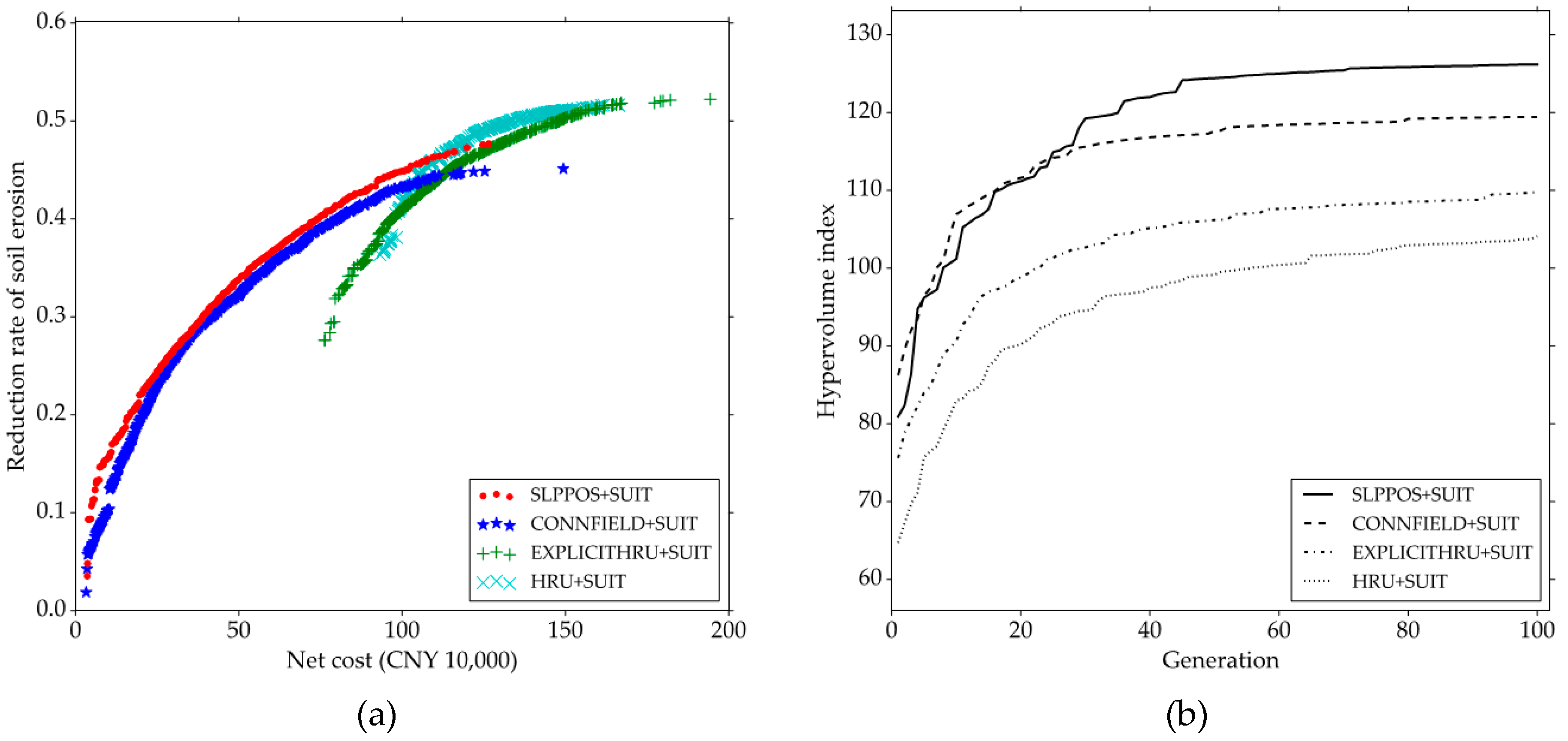
Figure 7 shows a comparison among four types of BMP configuration units applied with the SUIT strategy (i.e., SLPPOS+SUIT, CONNFIELD+SUIT, EXPLICITHRU+SUIT, and HRU+SUIT). The solution spaces of the spatial optimization of EXPLICITHRU+SUIT and HRU+SUIT were inclined to reach higher net costs, while SLPPOS+SUIT and CONNFIELD+SUIT comparatively concentrated on the solution spaces with low net costs (Figure 7a). HRU+SUIT and SLPPOS+SUIT obtained the most non-dominated solutions when the corresponding net costs were greater or less than about CNY 1.10 million, respectively. For HRU+SUIT and EXPLICITHRU+SUIT, the soil erosion reduction rate reached relative stability at about 0.52 when the corresponding net costs were greater than CNY 1.60 million (Figure 7a). The solutions of SLPPOS+SUIT obtained very similar hypervolume index values to those from CONNFIELD+SUIT in the first stage of optimization (about the first 35 generations) and then a higher hypervolume index during the following generations (Figure 7b). The EXPLICITHRU+SUIT and HRU+SUIT produced worse diversity than SLPPOS+SUIT and CONNFIELD+SUIT (Figure 7a). This phenomenon can also be observed from the lower hypervolume index from EXPLICITHRU+SUIT and HRU+SUIT (Figure 7b). The SLPPOS+SUIT, CONNFIELD+SUIT, EXPLICITHRU+SUIT, and HRU+SUIT reached stability at the 46th, 36th, 45th, and 60th generations, respectively (Figure 7b), among which the CONNFIELD+SUIT showed the best optimizing efficiency.
Since the HRUs and spatially explicit HRUs delineated in this study have a single landuse type for each spatial configuration unit, the non-effective configurations caused by BMP configuration units with multiple landuse types (e.g., hydrologically connected fields and slope position units) (Section 2.5) do not exist. Therefore, under the same parameter-settings of the optimization algorithm, EXPLICITHRU+SUIT and HRU+SUIT inherently generate more effective BMP configurations in locations within spatial configuration units than SLPPOS+SUIT and CONNFIELD+SUIT and thus result in a solution space with relatively high net costs.
With the best near-optimal Pareto solutions, the highest hypervolume index, and the satisfied optimizing efficiency, SLPPOS+SUIT obtained the best overall performance compared to the other three combinations with the SUIT strategy. This may be attributed to the knowledge used by the SUIT strategy for slope position units that considers not only suitable landuse types but also suitable slope positions of individual BMPs.
3.3. Comparison between Feasible BMP Configuration Units with the UPDOWN Strategy
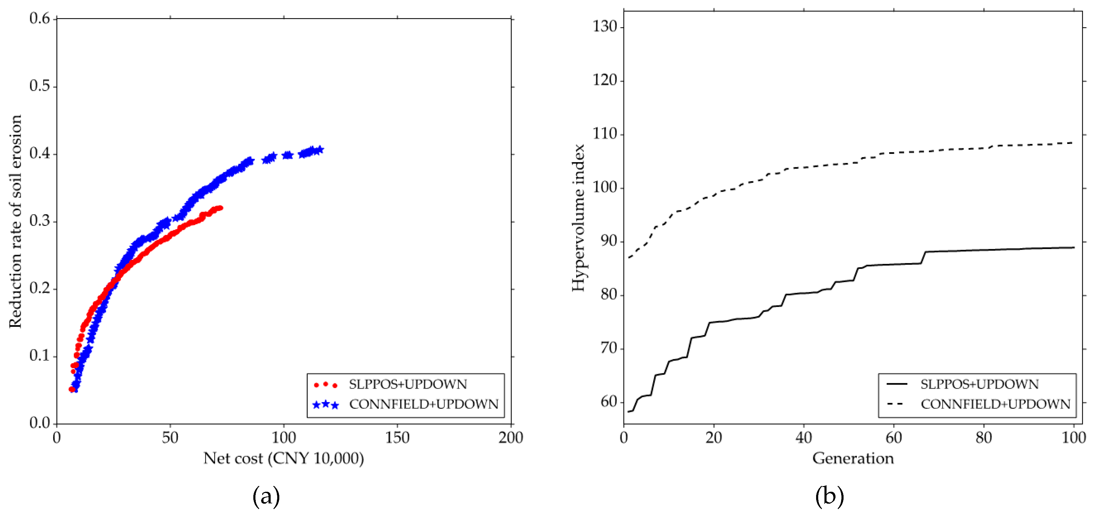
Figure 8 presents a comparison between two types of BMP configuration units applied with the UPDOWN strategy (i.e., SLPPOS+UPDOWN and CONNFIELD+UPDOWN). CONNFIELD+UPDOWN and SLPPOS+UPDOWN obtained most of their non-dominated solutions when the corresponding net costs were greater or less than about CNY 0.25 million, respectively (Figure 8a). SLPPOS+UPDOWN had a narrower solution space than CONNFIELD+UPDOWN and hence had worse diversity and a lower hypervolume index. CONNFIELD+UPDOWN showed a more steady hypervolume index trend with generations and better optimizing efficiency since it reached stability at the 39th generation which is lower than the 55th generation for SLPPOS+UPDOWN (Figure 8b). SLPPOS+UPDOWN reached slightly better hypervolume index stability after about the 70th generation, i.e., a slightly better convergence than CONNFIELD+UPDOWN.
Although the same strategy was applied, the upstream–downstream relationships of slope position units were built at the hillslope scale instead of the watershed scale of hydrologically connected fields. This means that the number of slope position units within one hillslope (i.e., three in this study) is the maximum number of genes allowed to be exchanged during crossover operation in NSGA-II (Section 2.6). This puts the SLPPOS+UPDOWN result in a slightly better convergence and worse diversity than CONNFIELD+UPDOWN. The non-dominated solutions with low net costs of SLPPOS+UPDOWN indicated the better cost-effectiveness of slope position units under a tight budget, while its worse cost-effectiveness with higher net costs than CONNFIELD+UPDOWN may imply that the UPDOWN strategy initially developed for hydrologically connected fields [5] is not the most effective strategy for slope position units.
3.4. Comparison among Different BMP Configuration Units with the Corresponding Optimal Configuration Strategies
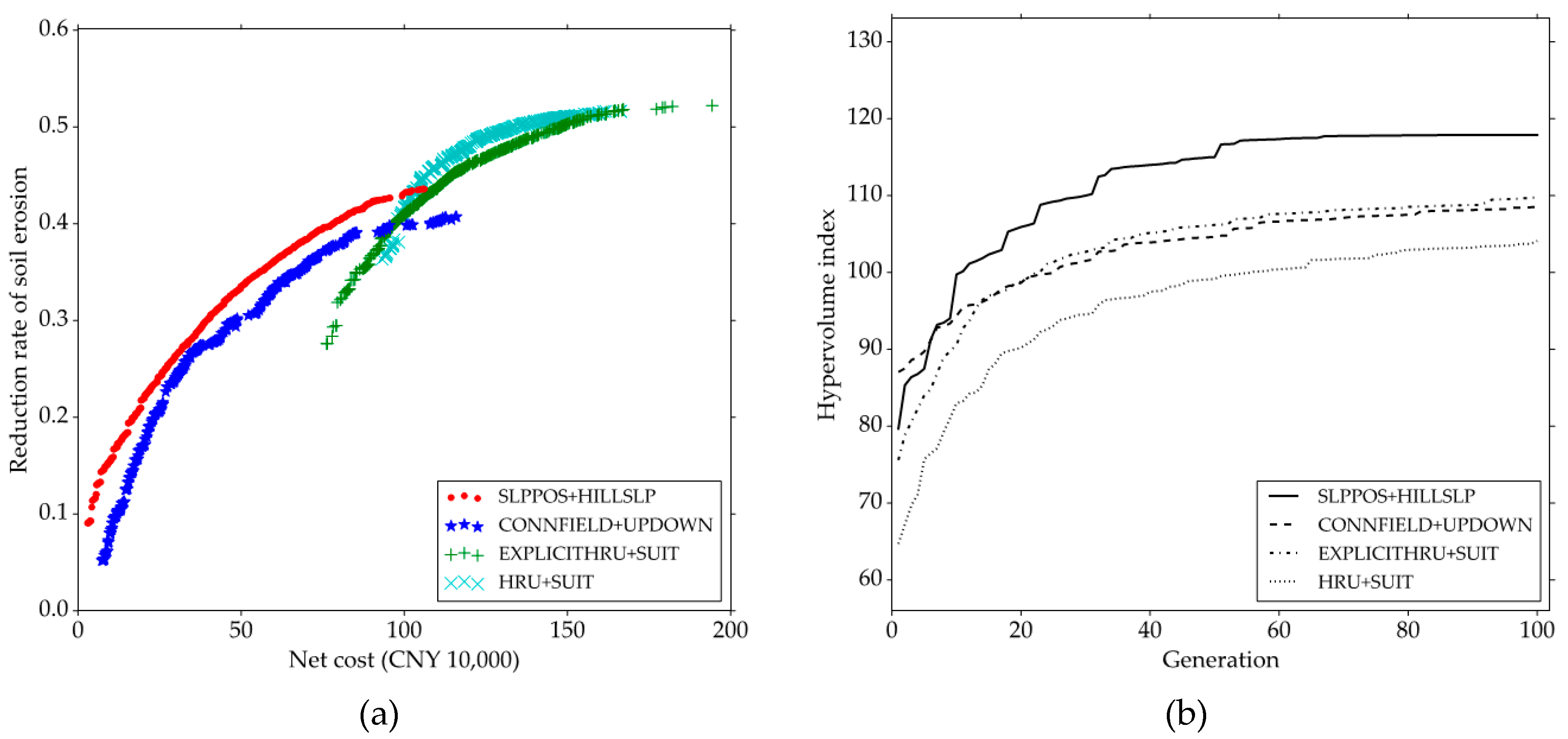
As shown in Figure 9a, HRU+SUIT and SLPPOS+HILLSLP generated the most effective non-dominated solutions when the corresponding net costs were greater and less than about CNY 1.0 million, respectively. According to the hypervolume index (Figure 9b), SLPPOS+HILLSLP reached the stable hypervolume index after the 37th generation, as well as the largest hypervolume index value, compared to the other three combinations. Thus, SLPPOS+HILLSLP showed the best optimizing efficiency. In summary, SLPPOS+HILLSLP showed the best overall performance (Figure 9), followed by EXPLICITHRU+SUIT and CONNFIELD+UPDOWN. Although HRU+SUIT had non-dominant solutions mostly at high net costs, it was still considered to have the worst overall performance because it produced the worst diversity, lowest hypervolume index, and slowest optimizing efficiency (i.e., reaching stability at the 60th generation; Section 3.2).
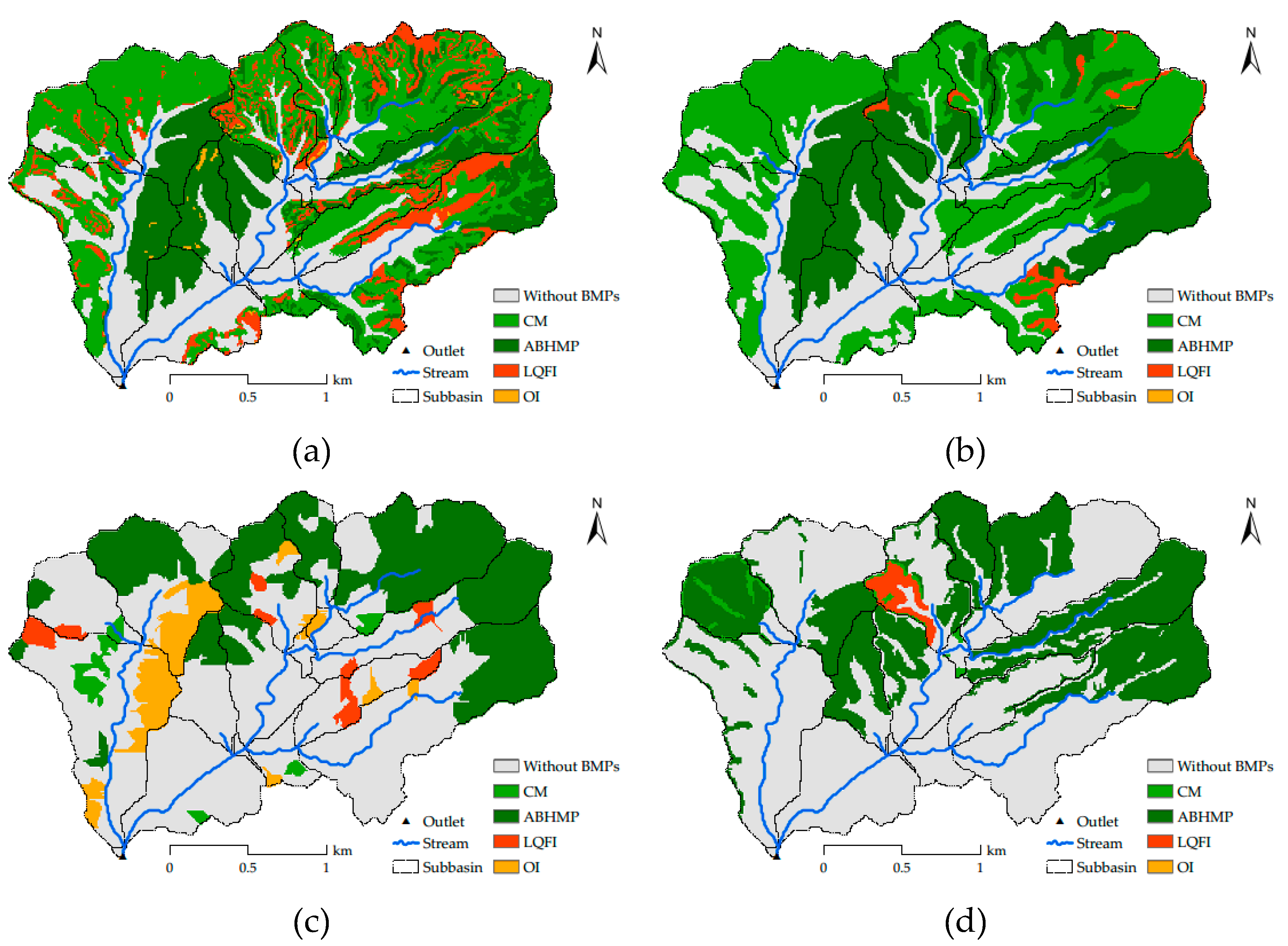
To compare the practicality of the spatial distribution of optimized BMP scenarios, four BMP scenarios (Figure 10) were selected in the overlapped solution space of the four combinations (i.e., at a soil erosion reduction rate of around 0.40 and net cost of CNY 0.70–1.20 million). The most fragmented spatial delineation of HRUs caused the worst practicality from the perspective of actual watershed management (Figure 10a). EXPLICITHRU+SUIT (Figure 10b) generated similar BMPs regions to HRU+SUIT (Figure 10a), but those from EXPLICITHRU+SUIT had a more concentrated and practical distribution of BMPs than those from HRU+SUIT. The BMP scenarios from CONNFIELD+UPDOWN required the highest net cost to achieve the same soil erosion reduction rate among these selected BMP scenarios, since CONNFIELD+UPDOWN selected the most expensive BMP (i.e., Orchard Improvement) for allocation (Figure 10c). With the adoption of the UPDOWN strategy and a smaller configuration area, the BMP scenario from CONNFIELD+UPDOWN (Figure 10c) achieved better practicality than that from EXPLICITHRU+SUIT (Figure 10b). With the SUIT and UPDOWN strategies, the lack of precise spatial relationships between BMPs and spatial positions at the hillslope scale may cause several inappropriate configurations (Figure 10a–c), e.g., the LQFI (Low-quality forest improvement) configured on ridge areas (Table 1), thus reducing the practicality of the BMP scenario from EXPLICITHRU+SUIT and CONNFIELD+UPDOWN. Depending on the HILLSLP strategy used to adopt BMP knowledge derived from the local experience of integrated watershed management, SLPPOS+HILLSLP concisely and precisely configured CM (Closing measures) and ABHMP (Arbor–bush–herb mixed plantation) on slope position units at the hillslope scale, e.g., CM-ABHMP on the ridge and backslope sequence, and also configured the BMP with the best overall effectiveness grade (i.e., ABHMP according to Table 3) on ridge and backslope. Thus, SLPPOS+HILLSLP obtained the best practicality with the lowest net cost among these selected BMP scenarios, followed by CONNFIELD+UPDOWN and EXPLICITHRU+SUIT.
4. Discussion
From a mathematical viewpoint, all feasible combinations of BMP configuration units and BMP configuration strategies generated effective near-optimal Pareto solutions (Figure 6, Figure 7, Figure 8 and Figure 9). Different delineations of BMP configuration units have different characteristics such as the number of units, the spatial distribution characteristics, and the spatial relationships with homogeneous functional units from the perspective of physical geography. These differences affect the characteristics of the generated BMP scenarios and the search spaces of spatial optimization, thus resulting in the different cost-effectiveness of near-optimal Pareto solutions and optimizing efficiency when applied with the same BMP configuration strategy (Section 3.1, Section 3.2 and Section 3.3).
BMP scenarios generated based on different kinds of BMP configuration knowledge had significant differences in the cost-effectiveness of the near-optimal Pareto solutions, optimizing efficiency, and the spatial distribution of the BMP scenarios. Using the strategies that adopt BMP configuration knowledge (i.e., the SUIT, UPDOWN, and HILLSLP strategies), those non-effective configurations generated by the random configuration strategy (Section 2.5) can be avoided for all BMP configuration units. Thus, with the BMP configuration constraint, better convergence, and worse diversity of near-optimal Pareto solutions were obtained, as well as overall lower values of hypervolume index and better optimizing efficiency (e.g., comparing Figure 7, Figure 8, and Figure 9 with Figure 6). Such phenomena could also be observed when the adopted knowledge extended from simple knowledge to knowledge on the spatial relationships between BMPs and spatial positions, i.e., from the SUIT strategy to the UPDOWN strategy or the HILLSLP strategy.
Besides the narrowed solution space of spatial optimization and improved optimizing efficiency, the adoption of domain (or expert) knowledge considering spatial relationships between BMPs and spatial positions, e.g., the UPDOWN and HILLSLP strategies in this study, can also facilitate the optimized BMP solutions with geographical and practical meanings (Section 3.4). The formal representation of such expert knowledge is often introduced according to the characteristics of specific BMP configuration units, which means that one BMP configuration strategy developed associated with one BMP configuration unit may not be effectively applied to another BMP configuration unit, e.g., the ineffective situation in which the UPDOWN strategy was applied to slope position units (Figure 8 and Figure 9).
The random strategy and simple knowledge-based strategy (e.g., the SUIT strategy) may obtain more effective near-optimal BMPs solutions at higher net costs than the strategies with knowledge on the spatial relationships between BMPs and spatial positions (e.g., the UPDOWN and HILLSLP strategies) (Figure 9a). However, the latter type of strategies can effectively represent the local experience of integrated watershed management with better practicality [2] and hence are more valuable for real applications, especially when the expert knowledge on the spatial relationships between BMPs and slope positions along a hillslope can be considered (Figure 10d).
5. Conclusions
This paper presents a comparison among the four main types of BMP configuration units (i.e., HRUs, spatially explicit HRUs, hydrologically connected fields, and slope position units) for watershed BMP scenarios optimization based on the same one distributed watershed model. Four BMP configuration strategies, adopting different kinds of BMP knowledge of the study area, were considered, i.e., the random configuration strategy, the strategy with knowledge on suitable landuse types/slope positions of individual BMPs, the strategy based on expert knowledge of upstream–downstream relationships [5], and the strategy with expert knowledge on the spatial relationships between BMPs and slope positions along the hillslope [2]. A total of 11 experiments of feasible combinations were conducted with the same optimization algorithm (i.e., NSGA-II) and then compared.
The comparison showed that different BMP configuration units applied with different configuration strategies had significant differences in near-optimal Pareto solutions, optimizing efficiency, and spatial distribution of BMP scenarios. Generally, the more the expert (or domain) knowledge was considered, the better the comprehensive cost-effectiveness and practicality of the optimized BMP scenarios, and the better the optimizing efficiency. Therefore, BMP configuration units that support the adoption of expert knowledge on the spatial relationships between BMPs and spatial locations [2,5] (i.e., hydrologically connected fields, and slope position units) are considered to be the most valuable spatial configuration units for watershed BMP scenarios optimization and integrated watershed management. Overall, using the slope position units as BMP configuration units with the HILLSLP strategy, the best comprehensive results of BMP scenarios optimization were obtained.
This study provided a useful reference for the spatial optimization of watershed BMP scenarios with multiple spatially explicit BMPs. For those spatially explicit BMPs, more BMP configuration knowledge derived from local management experiences should be summarized and adopted together with the feasible BMP configuration units for such knowledge (e.g., slope position units) during watershed BMP scenarios optimization.
Author Contributions
Conceptualization, L.-J.Z., C.-Z.Q., and A.-X.Z.; Methodology, L.-J.Z. and C.-Z.Q.; Software, L.-J.Z., J.L., and H.W.; Investigation, L.-J.Z.; Resources, J.L., C.-Z.Q., and A.-X.Z.; Writing—Original Draft Preparation, L.-J.Z. and C.-Z.Q.; Funding Acquisition, C.-Z.Q., and A.-X.Z.
Funding
The work reported was financially supported by the National Natural Science Foundation of China (No. 41871362 and 41431177), the National Key Technology R&D Program (No. 2013BAC08B03-4), the Chinese Academy of Sciences (No. XDA23100503), the Innovation Project of LREIS (No. O88RA20CYA), National Basic Research Program of China (Project No.: 2015CB954102), PAPD, and the Outstanding Innovation Team in Colleges and Universities in Jiangsu Province. Supports to A-Xing Zhu through the Vilas Associate Award, the Hammel Faculty Fellow Award, and the Manasse Chair Professorship from the University of Wisconsin-Madison are greatly appreciated.
Acknowledgments
The authors thank Zhi-Biao Chen for kindly permitting us to use his photos of the four types of BMPs considered in this study.
Conflicts of Interest
The authors declare no conflict of interest.
References
- Kalcic, M.M.; Frankenberger, J.; Chaubey, I. Spatial Optimization of Six Conservation Practices Using Swat in Tile-Drained Agricultural Watersheds. J. Am. Water Resour. Assoc. JAWRA 2015, 51, 956–972. [Google Scholar] [CrossRef]
- Qin, C.-Z.; Gao, H.-R.; Zhu, L.-J.; Zhu, A.-X.; Liu, J.-Z.; Wu, H. Spatial optimization of watershed best management practices based on slope position units. J. Soil Water Conserv. 2018, 73, 504–517. [Google Scholar] [CrossRef]
- Sahu, M.; Gu, R.R. Modeling the effects of riparian buffer zone and contour strips on stream water quality. Ecol. Eng. 2009, 35, 1167–1177. [Google Scholar] [CrossRef]
- Veith, T.L.; Wolfe, M.L.; Heatwole, C.D. Optimization Procedure for Cost Effective Bmp Placement at a Watershed Scale. J. Am. Water Resour. Assoc. JAWRA 2003, 39, 1331–1343. [Google Scholar] [CrossRef]
- Wu, H.; Zhu, A.-X.; Liu, J.; Liu, Y.; Jiang, J. Best Management Practices Optimization at Watershed Scale: Incorporating Spatial Topology among Fields. Water Resour. Manag. 2018, 32, 155–177. [Google Scholar] [CrossRef]
- Wang, X.; Amonett, C.; Williams, J.R.; Wilcox, B.P.; Fox, W.E.; Tu, M.-C. Rangeland watershed study using the Agricultural Policy/Environmental eXtender. J. Soil Water Conserv. 2014, 69, 197–212. [Google Scholar] [CrossRef]
- Duriancik, L.F.; Bucks, D.; Dobrowolski, J.P.; Drewes, T.; Eckles, S.D.; Jolley, L.; Kellogg, R.L.; Lund, D.; Makuch, J.R.; O’Neill, M.P. The first five years of the Conservation Effects Assessment Project. J. Soil Water Conserv. 2008, 63, 185A–197A. [Google Scholar] [CrossRef]
- Turpin, N.; Bontems, P.; Rotillon, G.; Bärlund, I.; Kaljonen, M.; Tattari, S.; Feichtinger, F.; Strauss, P.; Haverkamp, R.; Garnier, M.; et al. AgriBMPWater: Systems approach to environmentally acceptable farming. Environ. Model. Softw. 2005, 20, 187–196. [Google Scholar] [CrossRef]
- Xie, H.; Chen, L.; Shen, Z.; Xie, H.; Chen, L.; Shen, Z. Assessment of Agricultural Best Management Practices Using Models: Current Issues and Future Perspectives. Water 2015, 7, 1088–1108. [Google Scholar] [CrossRef]
- Arabi, M.; Govindaraju, R.S.; Hantush, M.M. Cost-effective allocation of watershed management practices using a genetic algorithm. Water Resour. Res. 2006, 42, W10429. [Google Scholar] [CrossRef]
- Gitau, M.W.; Veith, T.L.; Gburek, W.J. Farm-level optimization of BMP placement for cost-effective pollution reduction. Trans. ASAE 2004, 47, 1923–1931. [Google Scholar] [CrossRef]
- Maringanti, C.; Chaubey, I.; Arabi, M.; Engel, B. Application of a multi-objective optimization method to provide least cost alternatives for NPS pollution control. Environ. Manag. 2011, 48, 448–461. [Google Scholar] [CrossRef] [PubMed]
- Srivastava, P.; Hamlett, J.M.; Robillard, P.D.; Day, R.L. Watershed optimization of best management practices using AnnAGNPS and a genetic algorithm. Water Resour. Res. 2002, 38. [Google Scholar] [CrossRef]
- Chang, C.L.; Chiueh, P.T.; Lo, S.L. Effect of spatial variability of storm on the optimal placement of best management practices (BMPs). Environ. Monit. Assess. 2007, 135, 383–389. [Google Scholar] [CrossRef] [PubMed]
- Chichakly, K.J.; Bowden, W.B.; Eppstein, M.J. Minimization of cost, sediment load, and sensitivity to climate change in a watershed management application. Environ. Model. Softw. 2013, 50, 158–168. [Google Scholar] [CrossRef]
- Qiu, J.; Shen, Z.; Huang, M.; Zhang, X. Exploring effective best management practices in the Miyun reservoir watershed, China. Ecol. Eng. 2018, 123, 30–42. [Google Scholar] [CrossRef]
- Yang, G.X.; Best, E.P.H. Spatial optimization of watershed management practices for nitrogen load reduction using a modeling-optimization framework. J. Environ. Manag. 2015, 161, 252–260. [Google Scholar] [CrossRef]
- Panagopoulos, Y.; Makropoulos, C.; Mimikou, M. Decision support for diffuse pollution management. Environ. Model. Softw. 2012, 30, 57–70. [Google Scholar] [CrossRef]
- Rodriguez, H.G.; Popp, J.; Maringanti, C.; Chaubey, I. Selection and placement of best management practices used to reduce water quality degradation in Lincoln Lake watershed. Water Resour. Res. 2011, 47. [Google Scholar] [CrossRef]
- Band, L.E. Spatial hydrography and landforms. In GIS: Management Issues and Applications; Longley, P., Goodchild, M., Maguire, D., Rhind, D., Eds.; John Wiley & Sons: Hoboken, NI, USA, 1999; pp. 527–542. [Google Scholar]
- Jiang, P.; Anderson, S.H.; Kitchen, N.R.; Sadler, E.J.; Sudduth, K.A. Landscape and conservation management effects on hydraulic properties of a claypan-soil toposequence. Soil Sci. Soc. Am. J. 2007, 71, 803–811. [Google Scholar] [CrossRef]
- Mudgal, A.; Baffaut, C.; Anderson, S.H.; Sadler, E.J.; Thompson, A.L. APEX model assessment of variable landscapes on runoff and dissolved herbicides. Trans. ASABE 2010, 53, 1047–1058. [Google Scholar] [CrossRef]
- Arnold, J.G.; Srinivasan, R.; Muttiah, R.S.; Williams, J.R. Large area hydrologic modeling and assessment part I: Model development. J. Am. Water Resour. Assoc. JAWRA 1998, 34, 73–89. [Google Scholar] [CrossRef]
- Arnold, J.G.; Allen, P.M.; Volk, M.; Williams, J.R.; Bosch, D.D. Assessment of Different Representations of Spatial Variability on SWAT Model Performance. Trans. ASABE 2010, 53, 1433–1443. [Google Scholar] [CrossRef]
- Kalcic, M.M.; Chaubey, I.; Frankenberger, J. Defining Soil and Water Assessment Tool (SWAT) hydrologic response units (HRUs) by field boundaries. Int. J. Agric. Biol. Eng. 2015, 8, 69–80. [Google Scholar]
- Teshager, A.D.; Gassman, P.W.; Secchi, S.; Schoof, J.T.; Misgna, G. Modeling Agricultural Watersheds with the Soil and Water Assessment Tool (SWAT): Calibration and Validation with a Novel Procedure for Spatially Explicit HRUs. Environ. Manag. 2016, 57, 894–911. [Google Scholar] [CrossRef]
- Gaddis, E.J.B.; Voinov, A.; Seppelt, R.; Rizzo, D.M. Spatial Optimization of Best Management Practices to Attain Water Quality Targets. Water Resour. Manag. 2014, 28, 1485–1499. [Google Scholar] [CrossRef]
- Limbrunner, J.F.; Vogel, R.M.; Chapra, S.C.; Kirshen, P.H. Optimal Location of Sediment-Trapping Best Management Practices for Nonpoint Source Load Management. J. Water Resour. Plan. Manag. 2013, 139, 478–485. [Google Scholar] [CrossRef]
- Perez-Pedini, C.; Limbrunner, J.F.; Vogel, R.M. Optimal Location of Infiltration-Based Best Management Practices for Storm Water Management. J. Water Resour. Plan. Manag. 2005, 131, 441–448. [Google Scholar] [CrossRef]
- Qin, C.-Z.; Zhu, A.-X.; Shi, X.; Li, B.-L.; Pei, T.; Zhou, C.-H. Quantification of spatial gradation of slope positions. Geomorphology 2009, 110, 152–161. [Google Scholar] [CrossRef]
- Zhu, L.-J.; Zhu, A.-X.; Qin, C.-Z.; Liu, J.-Z. Automatic approach to deriving fuzzy slope positions. Geomorphology 2018, 304, 173–183. [Google Scholar] [CrossRef]
- Bieger, K.; Arnold, J.G.; Rathjens, H.; White, M.J.; Bosch, D.D.; Allen, P.M.; Volk, M.; Srinivasan, R. Introduction to SWAT+, A Completely Restructured Version of the Soil and Water Assessment Tool. JAWRA J. Am. Water Resour. Assoc. 2017, 53, 115–130. [Google Scholar] [CrossRef]
- Zhu, L.-J.; Liu, J.; Qin, C.-Z.; Zhu, A.-X. A modular and parallelized watershed modeling framework. Environ. Model. Softw. under review.
- Deb, K.; Pratap, A.; Agarwal, S.; Meyarivan, T. A fast and elitist multiobjective genetic algorithm: NSGA-II. IEEE Trans. Evol. Comput. 2002, 6, 182–197. [Google Scholar] [CrossRef]
- Chen, Z.-B.; Chen, Z.-Q.; Yue, H. Comprehensive Research on Soil and Water Conservation in Granite Red Soil Region: A Case Study of Zhuxi Watershed, Changting County, Fujian Province; Science Press: Beijing, China, 2013. (In Chinese) [Google Scholar]
- Shi, X.; Yang, G.; Yu, D.; Xu, S.; Warner, E.D.; Petersen, G.W.; Sun, W.; Zhao, Y.; Easterling, W.E.; Wang, H. A WebGIS system for relating genetic soil classification of China to soil taxonomy. Comput. Geosci. 2010, 36, 768–775. [Google Scholar] [CrossRef]
- Arnold, J.G.; Kiniry, J.R.; Srinivasan, R.; Williams, J.R.; Haney, E.B.; Neitsch, S.L. Soil and Water Assessment Tool 2012 Input/Output Documentation; Texas Water Resources Institute: College Station, TX, USA, 2012. [Google Scholar]
- Chen, S.; Zha, X. Evaluation of soil erosion vulnerability in the Zhuxi watershed, Fujian Province, China. Nat. Hazards 2016, 82, 1589–1607. [Google Scholar] [CrossRef]
- Dile, Y.T.; Daggupati, P.; George, C.; Srinivasan, R.; Arnold, J. Introducing a new open source GIS user interface for the SWAT model. Environ. Model. Softw. 2016, 85, 129–138. [Google Scholar] [CrossRef]
- Chen, Z.-Q.; Chen, Z.-B.; Bai, L.; Zeng, Y. A catastrophe model to assess soil restoration under ecological restoration in the red soil hilly region of China. Pedosphere 2017, 27, 778–787. [Google Scholar] [CrossRef]
- Fujian Soil and Water Conservation Monitoring Station; Fujian Agriculture and Forestry University; Fujian Normal University; Changting Soil and Water Conservation Monitoring Station. Monitoring Report of Soil and Water Loss in Changting County; Fuzhou, Fujian, China, 2010. (In Chinese) [Google Scholar]
- Liu, Y.; Engel, B.A.; Flanagan, D.C.; Gitau, M.W.; McMillan, S.K.; Chaubey, I.; Singh, S. Modeling framework for representing long-term effectiveness of best management practices in addressing hydrology and water quality problems: Framework development and demonstration using a Bayesian method. J. Hydrol. 2018, 560, 530–545. [Google Scholar] [CrossRef]
- Liu, J.; Zhu, A.-X.; Qin, C.-Z.; Wu, H.; Jiang, J. A two-level parallelization method for distributed hydrological models. Environ. Model. Softw. 2016, 80, 175–184. [Google Scholar] [CrossRef]
- Williams, J.R. Sediment-yield prediction with universal equation using runoff energy factor. In Present and Prospective Technology for Predicting Sediment Yield and Sources; U.S. Department of Agriculture: Washington, DC, USA, 1975; Volume ARS-S-40, pp. 244–252. [Google Scholar]
- Morris, M.D. Factorial sampling plans for preliminary computational experiments. Technometrics 1991, 33, 161–174. [Google Scholar] [CrossRef]
- Moriasi, D.N.; Arnold, J.G.; Van Liew, M.W.; Bingner, R.L.; Harmel, R.D.; Veith, T.L. Model evaluation guidelines for systematic quantification of accuracy in watershed simulations. Trans. ASABE 2007, 50, 885–900. [Google Scholar] [CrossRef]
- Zitzler, E.; Thiele, L. Multiobjective evolutionary algorithms: A comparative case study and the strength Pareto approach. IEEE Trans. Evol. Comput. 1999, 3, 257–271. [Google Scholar] [CrossRef]
- Zitzler, E.; Thiele, L.; Laumanns, M.; Fonseca, C.M.; da Fonseca, V.G. Performance assessment of multiobjective optimizers: An analysis and review. IEEE Trans. Evol. Comput. 2003, 7, 117–132. [Google Scholar] [CrossRef]
Figure 1.
Schematic diagram of spatial discretization of a watershed at different levels (such as sub-basins, hydrologic response units (HRUs), farms, hydrologically connected fields, slope position units, and grid cells) and the corresponding best management practice (BMP) scenario examples after allocating multiple types of BMPs based on different kinds of expert knowledge.

Figure 2.
Framework comparing the effects of different BMP configuration units for the spatial optimization of watershed BMP scenarios in this study (extended from [2]).
Figure 2.
Framework comparing the effects of different BMP configuration units for the spatial optimization of watershed BMP scenarios in this study (extended from [2]).

Figure 3.
Map of the Youwuzhen watershed in Fujian Province, China (adapted from [2]).
Figure 3.
Map of the Youwuzhen watershed in Fujian Province, China (adapted from [2]).

Figure 4.
Map of landuse in the study area.

Figure 5.
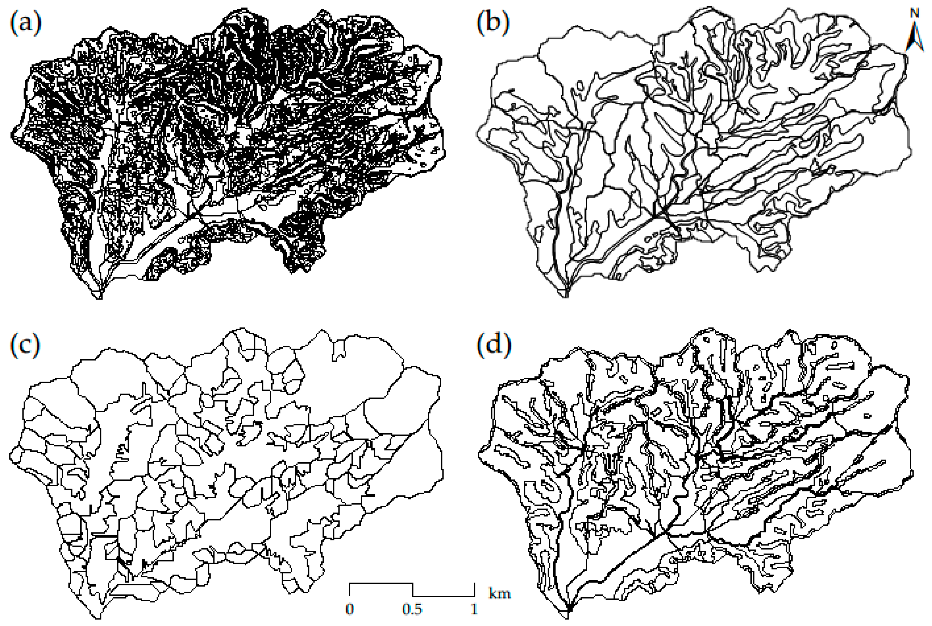
Delineations of BMP configuration units of the Youwuzhen watershed: (a) HRUs; (b) spatially explicit HRUs; (c) hydrologically connected fields; (d) slope position units.
Figure 5.
Delineations of BMP configuration units of the Youwuzhen watershed: (a) HRUs; (b) spatially explicit HRUs; (c) hydrologically connected fields; (d) slope position units.

Figure 6.
Comparisons among four types of BMP configuration units applied with the random configuration (RAND) strategy: (a) near-optimal Pareto solutions of the 100th generation and, (b) the hypervolume index with generations.
Figure 6.
Comparisons among four types of BMP configuration units applied with the random configuration (RAND) strategy: (a) near-optimal Pareto solutions of the 100th generation and, (b) the hypervolume index with generations.

Figure 7.
Comparisons among four types of BMP configuration units applied with the suitable landuse types/slope positions of individual BMPs (SUIT) strategy: (a) near-optimal Pareto solutions of the 100th generation, and (b) the hypervolume index with generations.
Figure 7.
Comparisons among four types of BMP configuration units applied with the suitable landuse types/slope positions of individual BMPs (SUIT) strategy: (a) near-optimal Pareto solutions of the 100th generation, and (b) the hypervolume index with generations.

Figure 8.
Comparisons between two types of BMP configuration units applied with the UPDOWN strategy: (a) near-optimal Pareto solutions of the 100th generation, and (b) the hypervolume index with generations.
Figure 8.
Comparisons between two types of BMP configuration units applied with the UPDOWN strategy: (a) near-optimal Pareto solutions of the 100th generation, and (b) the hypervolume index with generations.

Figure 9.
Comparisons among four types of BMP configuration units applied with the corresponding optimal configuration strategies: (a) near-optimal Pareto solutions of the 100th generation, and (b) the hypervolume index changed with generations.
Figure 9.
Comparisons among four types of BMP configuration units applied with the corresponding optimal configuration strategies: (a) near-optimal Pareto solutions of the 100th generation, and (b) the hypervolume index changed with generations.

Figure 10.
Comparison of the spatial distribution of selected BMP scenarios of the 100th generation from four types of BMP configuration units applied with the corresponding optimal strategies: (a) one HRU+SUIT scenario with a soil erosion reduction rate of 0.41 and a net cost of CNY 0.98 million; (b) one EXPLICIT+SUIT scenario with a soil erosion reduction rate of 0.40 and a net cost of CNY 0.97 million; (c) one CONNFIELD+UPDOWN scenario with a soil erosion reduction rate of 0.40 and a net cost of CNY 1.08 million; and (d) one SLPPOS+HILLSLP scenario with a soil erosion reduction rate of 0.40 and a net cost of CNY 0.78 million.


Table 1.
Brief descriptions of the four BMPs considered in this study (adapted from [2,40]; photos from [35]).
| BMP | Photo | Brief Description |
|---|---|---|
| Closing measures (CM) |  | Closing the ridge area and/or upslope positions from human disturbance (e.g., ban on felling tree and grazing) to facilitate afforestation. |
| Arbor–bush–herb mixed plantation (ABHMP) |  | Planting trees (e.g., Schima superba and Liquidambar formosana), bushes (e.g., Lespedeza bicolor), and herbs (e.g., Paspalum wettsteinii) in level trenches with compound fertilizer on hillslopes. |
| Low-quality forest improvement (LQFI) |  | Improving the infertile forest located in the upslope and steep backslope positions by applying compound fertilizer to the hole with a size of 40 cm × 40 cm × 40 cm in the uphill position of crown projection. |
| Orchard improvement (OI) |  | Improving orchards on the middle and down slope positions under better water and fertilizer conditions by constructing level terraces, drainage ditches, storage ditches, irrigation facilities, and roads, planting economic fruit, and interplanting grasses and Fabaceae (Leguminosae) plants. |
Table 2.
Environmental effectiveness and cost-benefit knowledge of the four BMPs (CM = Closing measures, ABHMP = Arbor–bush–herb mixed plantation, LQFI = Low-quality forest improvement, OI = Orchard improvement) (adapted from [2]).
Table 2.
Environmental effectiveness and cost-benefit knowledge of the four BMPs (CM = Closing measures, ABHMP = Arbor–bush–herb mixed plantation, LQFI = Low-quality forest improvement, OI = Orchard improvement) (adapted from [2]).
| BMP | Environmental Effectiveness 1 | Cost-Benefit (CNY 10,000/km2) | |||||||
|---|---|---|---|---|---|---|---|---|---|
| OM | BD | PORO | SOL_K | USLE_K | USLE_P | Initial | Maintain/yr | Benefit/yr | |
| CM | 1.22 | 0.98 | 1.02 | 0.81 | 1.01 | 0.90 | 15.5 | 1.5 | 2.0 |
| ABHMP | 1.45 | 0.93 | 1.07 | 1.81 | 0.82 | 0.50 | 87.5 | 1.5 | 6.9 |
| LQFI | 1.05 | 0.87 | 1.13 | 1.71 | 1.71 | 0.50 | 45.5 | 1.5 | 3.9 |
| OI | 2.05 | 0.96 | 1.03 | 1.63 | 1.63 | 0.75 | 420 | 20 | 60.3 |
1 Environmental effectiveness of BMPs includes soil property parameters (i.e., OM = organic matter, BD = bulk density, PORO = total porosity, and SOL_K = soil hydraulic conductivity) and universal soil loss equation (USLE) factors (i.e., USLE_K = soil erodibility factor and USLE_P = conservation practice factor). Values in this column represent relative changes (i.e., multiplying) to the original property values and thus have no units.
Table 3.
Suitable landuse types/slope positions and the overall environmental effectiveness grade of the four BMPs (CM = Closing measures, ABHMP = Arbor–bush–herb mixed plantation, LQFI = Low-quality forest improvement, OI = Orchard improvement) (adapted from [2]).
Table 3.
Suitable landuse types/slope positions and the overall environmental effectiveness grade of the four BMPs (CM = Closing measures, ABHMP = Arbor–bush–herb mixed plantation, LQFI = Low-quality forest improvement, OI = Orchard improvement) (adapted from [2]).
| BMP | Suitable Landuse Types | Suitable Slope Positions | Effectiveness Grade |
|---|---|---|---|
| CM | forest | ridge, backslope | 3 |
| ABHMP | forest, orchard | ridge, backslope, and valley | 5 |
| LQFI | forest | backslope | 4 |
| OI | forest, orchard | valley | 4 |
Table 4.
The calibration (2014–2015) and validation (2013) results of the baseline scenario by the Spatially Explicit Integrated Modeling System (SEIMS)-based watershed model. (NSE = Nash–Sutcliffe Efficiency, RSR = Root mean Square error–standard deviation Ratio, PBIAS = Percent BIAS).
Table 4.
The calibration (2014–2015) and validation (2013) results of the baseline scenario by the Spatially Explicit Integrated Modeling System (SEIMS)-based watershed model. (NSE = Nash–Sutcliffe Efficiency, RSR = Root mean Square error–standard deviation Ratio, PBIAS = Percent BIAS).
| Constituent | Calibration Period (2014–2015) | Validation Period (2013) | ||||
|---|---|---|---|---|---|---|
| NSE | RSR | PBIAS (%) | NSE | RSR | PBIAS (%) | |
| Streamflow (m3 s−1) | 0.50 | 0.71 | 13.55 | 0.57 | 0.65 | −14.71 |
| Sediment export (kg) | 0.30 | 0.84 | 13.93 | 0.45 | 0.74 | −42.39 |
© 2019 by the authors. Licensee MDPI, Basel, Switzerland. This article is an open access article distributed under the terms and conditions of the Creative Commons Attribution (CC BY) license (http://creativecommons.org/licenses/by/4.0/).
Share and Cite
MDPI and ACS Style
Zhu, L.-J.; Qin, C.-Z.; Zhu, A.-X.; Liu, J.; Wu, H. Effects of Different Spatial Configuration Units for the Spatial Optimization of Watershed Best Management Practice Scenarios. Water 2019, 11, 262. https://doi.org/10.3390/w11020262
AMA Style
Zhu L-J, Qin C-Z, Zhu A-X, Liu J, Wu H. Effects of Different Spatial Configuration Units for the Spatial Optimization of Watershed Best Management Practice Scenarios. Water. 2019; 11(2):262. https://doi.org/10.3390/w11020262
Chicago/Turabian StyleZhu, Liang-Jun, Cheng-Zhi Qin, A-Xing Zhu, Junzhi Liu, and Hui Wu. 2019. "Effects of Different Spatial Configuration Units for the Spatial Optimization of Watershed Best Management Practice Scenarios" Water 11, no. 2: 262. https://doi.org/10.3390/w11020262
Note that from the first issue of 2016, this journal uses article numbers instead of page numbers. See further details here.