Performance of A Two-Dimensional Hydraulic Model for the Evaluation of Stranding Areas and Characterization of Rapid Fluctuations in Hydropeaking Rivers

Abstract

Extreme, short-duration fluctuations caused by hydropeaking occurs when hydropower is regulated to cover demand peaks in the electricity market. Such rapid dewatering processes may have a high impact on the downstream biological conditions, particularly related to stranding of fish and other species. The present work analyzes these fluctuations using a two-dimensional unsteady hydraulic modelling approach for quantification of two important hydro-morphological factors on fish stranding risk: the variation in wetted area and the dewatering ramping rate. This approach was applied on the two-kilometer-long reach of Storåne downstream of the Hol 1 power plant, where topo bathymetric LiDAR (Light Detection and Ranging) data was available providing a high-resolution digital elevation model. Based on this model, hydraulic conditions could be simulated in high detail allowing for an accurate assessment of the hydro morphological factors. Results show the dried area distribution at different flows and dewatering ramping rates. The attenuation of the water level fluctuation due to the damping effect along the river reach controls the dewatering rate. We recommend an alternative scenario operation which can reduce the impact of the peaking operation and estimate the operational mitigation cost. We find that the modelling based on the fine resolution grid provides new opportunities in assessing effects of hydropower regulations on the ecosystem.

1. Introduction

By 2050, the European Union (EU) should cut greenhouse gas emissions to 80% below 1990 levels [1]. Electricity generation, in all its forms, contributes to over a third of the global energy-related CO₂ emissions and therefore energy transition is a fundamental step towards sustainability. In this frame, hydropower is expected to play a key role to balance the load of other renewable resources [2]. Norway has approximately half of the hydropower reservoir capacity in Europe [3], and thereby a large potential for load balancing. Short-term changes in electricity demands, for instance because of intermittent electricity generation from solar and wind energy, will increase hydropeaking production leading to higher fluctuations in discharge and water levels. In addition, the implementation of the Water Framework Directive and the revision of hydropower licenses in Norway in 2022 [4] may lead to new environmental restrictions in regulated rivers. Consequently, information for improved decision making is necessary.

Ecological impacts of hydropeaking have been reviewed in several studies [5,6,7,8]. Among the ecological impacts are the drifting of macroinvertebrates [9,10], the effects on riverine plants [11] and the stranding of juvenile fish [12]. Fish stranding can be encountered whenever fish are restricted to poor habitat due to physical separation from a main body of water because of flow decrease [13]. There are several studies on fish stranding, particularly salmon and brown trout [7,12,14,15,16]. These species, unable to follow the recessive water line when a rapid decrease occurs, may strand on flat river banks or be trapped in pools disconnected from the main channel which are gradually dewatered. Although fish stranding experiments have been performed in laboratories [7,16] or in limited areas in rivers [12], few studies exist on a larger scale in rivers about stranding. Hedger et al. [17] developed an individually based population model that showed how hydropeaking-induced stranding mortality affects Atlantic salmon population along multiple generations.

Modelling and quantification of ecological effect of hydropeaking interactions are a main issue to select appropriate mitigation methods to avoid stranding. The Center for Environmental Design of Renewable Energy (CEDREN) developed in the project Envipeak guidelines for the evaluation of hydropeaking impacts directed at river management [5]. These are from now on referred to as the Envipeak guidelines. Casas-Mulet et al. [18], evaluated the use of a one-dimensional hydraulic model for the estimation of potential stranding areas. They found that detailed cross-sectional data is needed to accurately predict dewatered areas. Two-dimensional models have been applied to assess the stranding fish. Tuhtan et al. [19] combined hydrodynamic and habitat modelling, showing this to be an useful tool to identify critical ranges. Vanzo et al. [20] outlined the advantages of adopting a two-dimensional unsteady approach, which allow a more accurate description of wetted area variation and dewatering ramping rate. Lack of precise geometrical data can be an issue in hydraulic modelling, but in recent years topo-bathymetric light detection and ranging (LiDAR) data has provided a high-resolution source used for modelling and monitoring of hydro-morphological units (mesohabitat scale) including the consequences for the target fish species [21].

There are three principal methods to reduce hydropower impacts. The first one is operational measures, which focus on changing the performance of energy production, for example by imposing a minimum flow or changing the operational time of the turbines [22] with the consequence of reducing the income of the hydropower plant operator [23]. The second one is construction measures that decrease the hydropeaking flows downstream of the outlet by building dikes, basins, bypass tunnels or other structures, usually measures with high investment costs. Finally, morphological measures, that aim to restore a good level of naturalness of the river with a consequent improvement of the area suitable for the biotic system, also with high investment costs. Recent studies show that combining morphological, operational and construction measures could help to find a balance between production losses, investment costs and ecological benefits [23,24].

The aim of this paper is to predict potential stranding areas utilizing a 2D hydraulic model on Storåne River in Hallingdal, Norway, where the community of brown trout (Salmo trutta) is strongly reduced downstream of the outlet of the Hol 1 hydropower plant [25]. Specific objectives were as follows: (i) characterize peaking operation; (ii) assess the performance of a 2D model based on LiDAR data for stranding area computation; (iii) evaluate stranding areas based on two main hydro-morphological features: wetted area and the dewatering ramping rates based on Envipeak guidelines [5] and (iv) propose an alternative operation procedure for mitigation.

2. Materials and Methods

2.1. Study Site

The study area is the river Storåne between the outlet of Hol 1 power plant and Hovsfjorden (Figure 1), located in the Hol Municipality in Buskerud county in Norway. It is a part of E-CO Energi’s regulation system in the Hallingdal region. The first 400 meters downstream of the outlet is a humanmade stone laid trapezoidal channel, whereas the rest of the river is a natural braided river section with several side channels forming three main islands, Ellingøyne, Gjerdeøyne and Mørkaøyne. The river width ranges from 10–150 meters. The discharge depends on the production in Hol 1 in addition to residual flow from the bypassed river section upstream of the outlet. Storåne is a clear, relatively shallow (mean depth <1 m) mountain stream. The mesohabitat varies between glide and riffle with some steep sections. The total river length that are accessible for trout migrating up from Lake Hovsfjorden is 8.1 km, and the reach affected by hydropeaking is 2.0 km.

Technical Details for Hol 1 Power Station

Hol 1 Hydro Power station was built in the period 1940–1956. There are four Francis turbines in two groups; Hol 1 Urunda and Hol 1 Votna. The two turbines in the Urunda group each have a capacity of 53 MW and are connected to the Strandavatn reservoir with a storage capacity of 619.8 million m³. The turbines in the Votna group have a 57 MW capacity each and are connected to a small reservoir (Varaldset) that is connected with three larger reservoirs. The total storage capacity for the Votna group is 229.7 million m³. The average production in Hol 1 is 750 GWh per year.

Hol 1 power station is a large hydropower station that is delivering power grid stabilization (Hz and Volt) on request from the national grid, and there has been an increase in the request for balancing power in the period 2010–2017. This will increase in the future as more intermittent power such as small-scale run-of-the-river hydropower and solar are constructed and start delivering to the grid [26].

2.2. Characterization of Rapid Fluctuations

The characterization of the peaking events was made by COSH-Tool, developed by SINTEF Energy Research, NO-7465 Trondheim, Norway [27]. In contrast with similar analyses, it separates peaking events into rapid increases and rapid decreases. It also analyses daylight conditions during peaking events and calculates the parameters for a specific season of the year defined by the user [27]. The tool characterizes the fluctuations in flow based on three parameters: magnitude, timing and frequency. Discharge data are needed as an input for the program.

E-CO Energi provided time series of discharge every hour from 2010 to 2017. The station is located 100 meters downstream of the outlet and it measures the flow through Hol 1 power station plus residual flow from Storåne. An upper limit was used in COSH-Tool to remove the effect of the few natural floods observed in the river.

2.3. River Geometry

The geometry input for the 2D hydraulic model is based on airborne light detection and ranging (LiDAR) data, a remote sensing technique for mapping relatively shallow water bodies, which is increasingly used for topo bathymetric surveys providing a high-quality digital elevation model [21]. In Storåne, LiDAR bathymetry reached an 8 m depth [28]. It is a fast method for collecting high density data, covering rivers of 15–20 km in a few hours. The high level of detail results in a large amount of data, which requires extensive processing before it can be used. The data was delivered as LAZ files, a special type of compression just for LiDAR data. I was deliver by Airborn Hydro Mapping (AHM), Austria, who carried out the flights and data processing. The coordinate system is European Terrestrial Reference System 1989 (ETRS 1989) with ellipsoidal height which, in Storåne, is 44.4 m over the NN2000 reference system normally used in Norway. Data were imported into ArcGIS 10.5, (Environmental Systems Research Institute, California, USA) to create the digital elevation model (DEM) that was used in the hydraulic model.

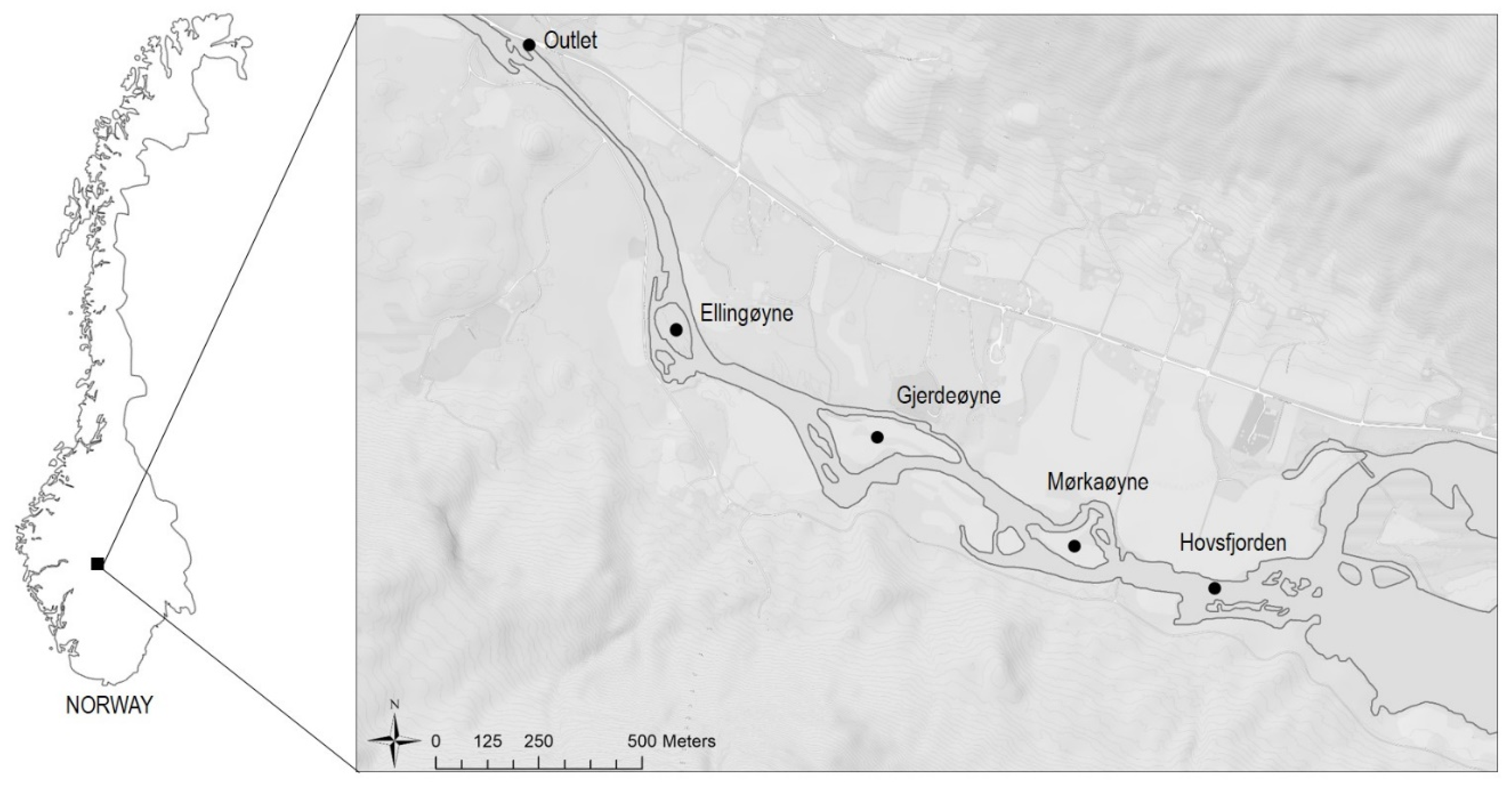
The entire length of the study site from the outlet to Hovsfjord is 2 km and the total mapped length was 2.6 km including areas upstream and downstream of the study site not used in the model. The number of points recorded were more than 82 million with an accuracy of 6 cm in the XY plane and mean error of 3 cm in elevation [28]. The point cloud has different density areas. The density affected mainly the water depth with fewer points in the deep areas of the river. Based on this, a DEM with a resolution of 0.5 × 0.5 m was created to ensure that in every square of the DEM there is a point. The DEM could be made finer in areas where point density is higher but we considered our DEM appropriate for the aim of the study.

2.4. Scenarios

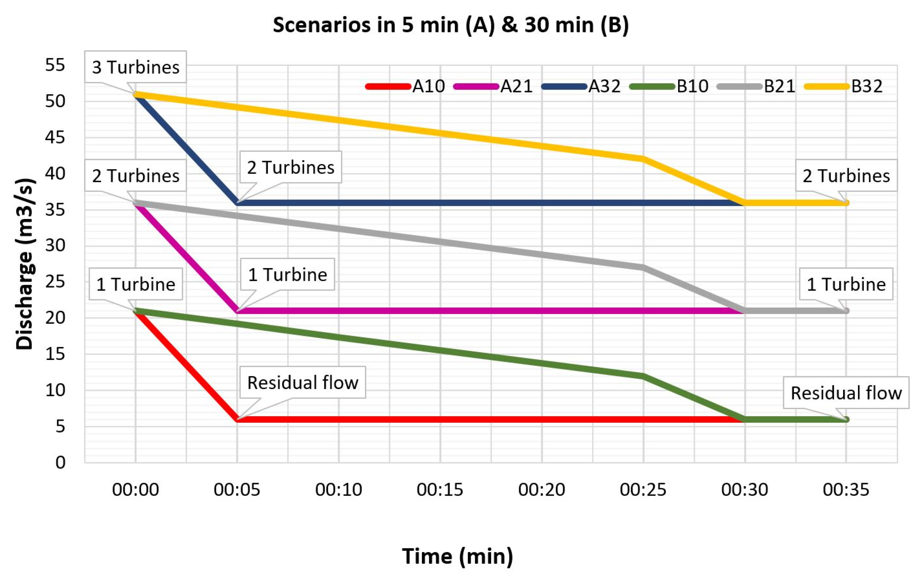
A series of different turbine shut down scenarios have been designed to simulate and quantify the stranding risk areas downstream Hol 1 power plant. The station has four turbines, each one with a capacity of 15 m³/s. The residual flow in the river was set at 6 m³/s representing the 5-percentile flow.

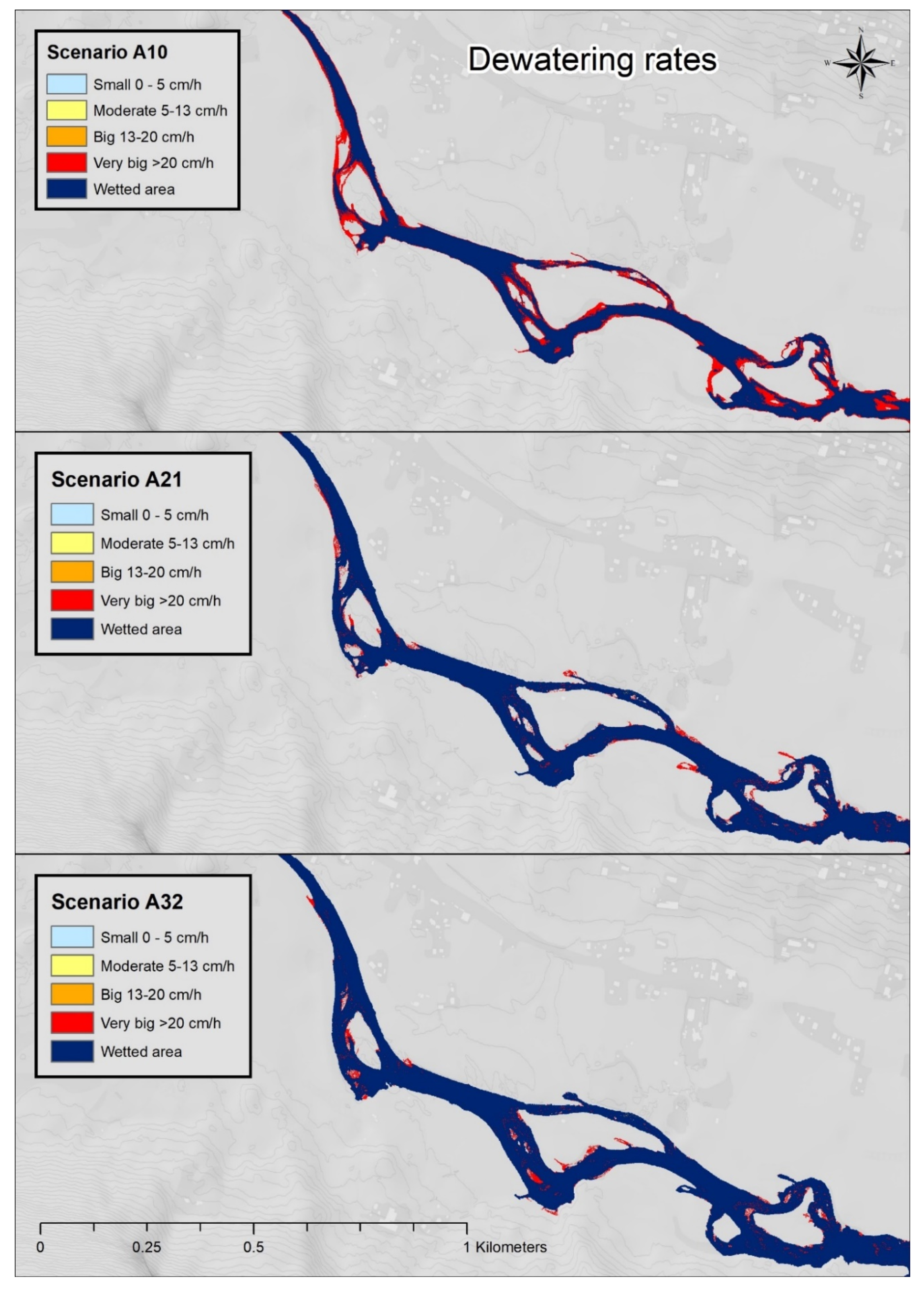
Currently the typical dewatering scenario is a discharge decrease of 15 m³/s in 5 minutes for each turbine. This configuration represents Scenarios A in the study. There are three different scenarios A: A10, the power plant decreases the production from one turbine (21 m³/s) to zero turbines (residual flow of 6 m³/s); scenario A21, the power plant decreases the production from two turbines (36 m³/s) to one turbine (21 m³/s) and scenario A32, the discharge goes from three turbines (51 m³/s) to two turbines (36 m³/s) (Figure 2). The scenario where we go from four turbines to three turbines was considered for the wetted areas only and not for dewatering scenarios since this is over the 95-percentile discharge and therefore not critical for the stranding. The full production scenario of 66 m³/s, is considered as the base line for the calculation of dry areas.

All the possible scenario combinations can be obtained by overlapping the simplified scenarios that are proposed in the previous paragraph, for instance, going from three to zero turbines in 5 minutes will be obtained by overlapping scenarios A32, A21 and A10.

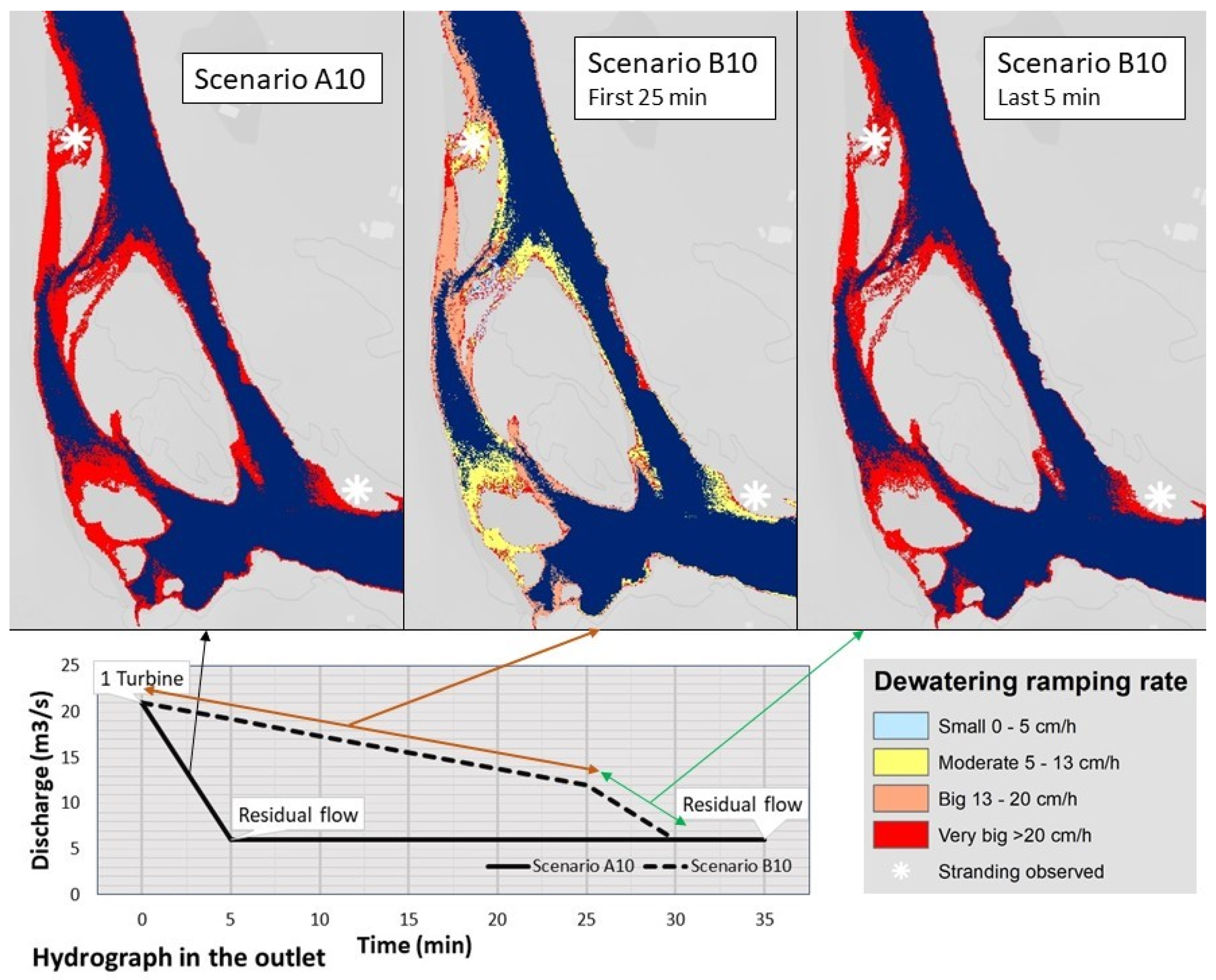
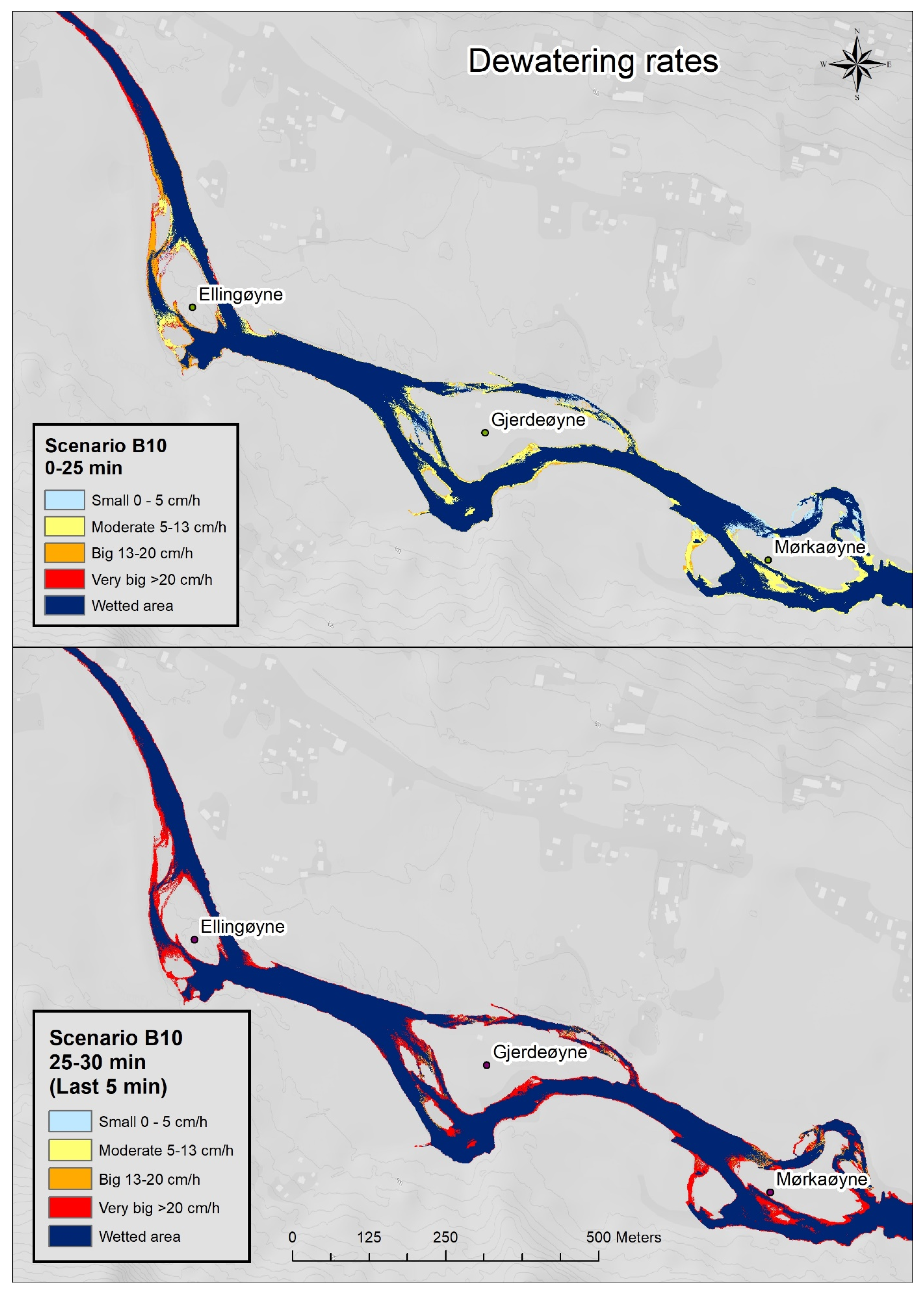
We designed a different alternative for each of these scenarios, called Scenarios B (Figure 2). They are designed so that the turbine goes from full production to 40% production in 25 min and then stops in 5 min for a full shut down time of 30 min. The need for the last fast drop is due to the manufacturer‘s restrictions, the turbines cannot operate at values under 40% of max discharge (B. 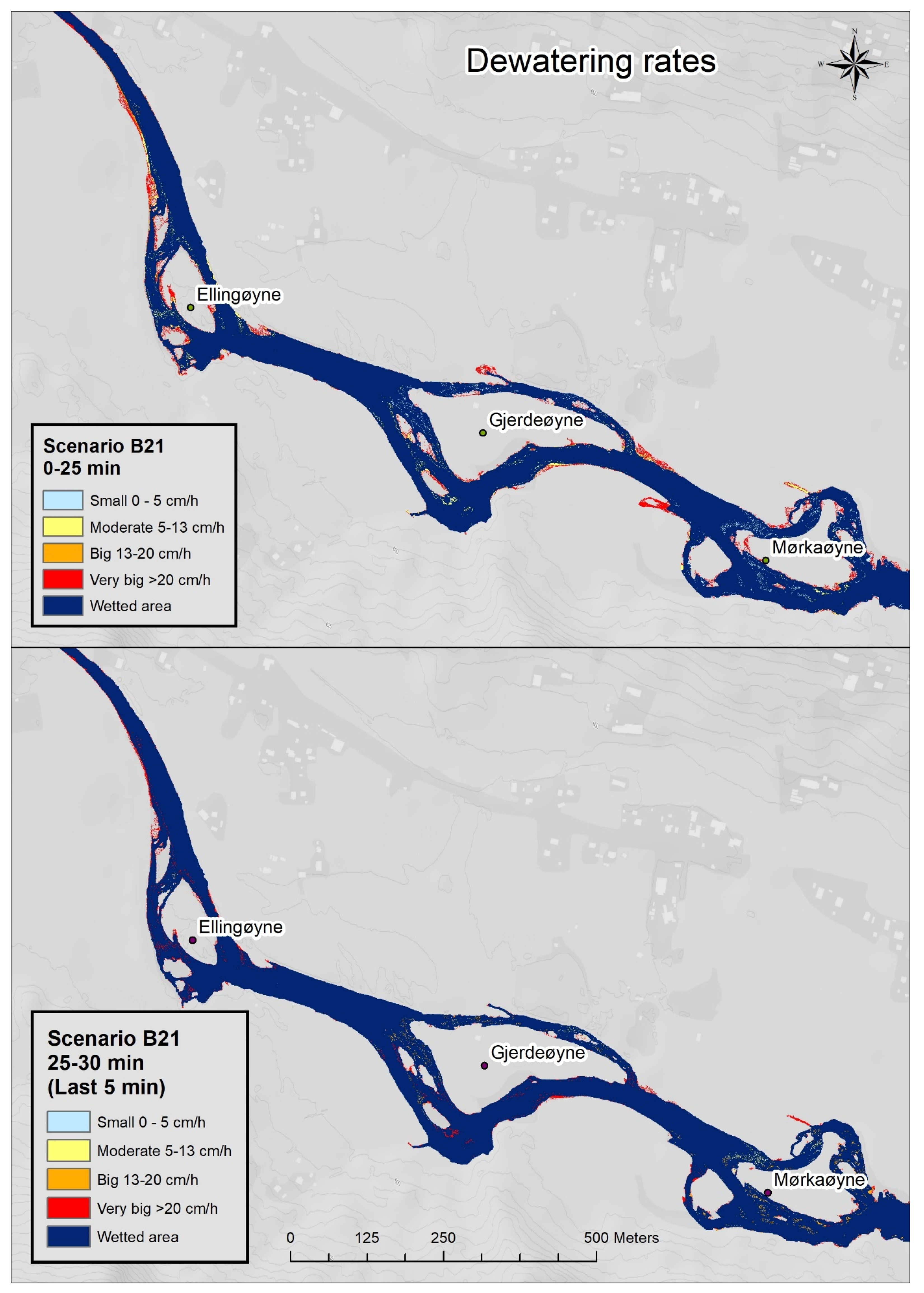Dønnum, personal comunication B10 is designed to go from one turbine to zero turbine in 30 minutes, in the first 25 minutes it decreases to 40% of turbine capacity (12 m³/s) and in the last 5 minutes the turbine is completely stopped and we only have residual flow (6 m³/s). 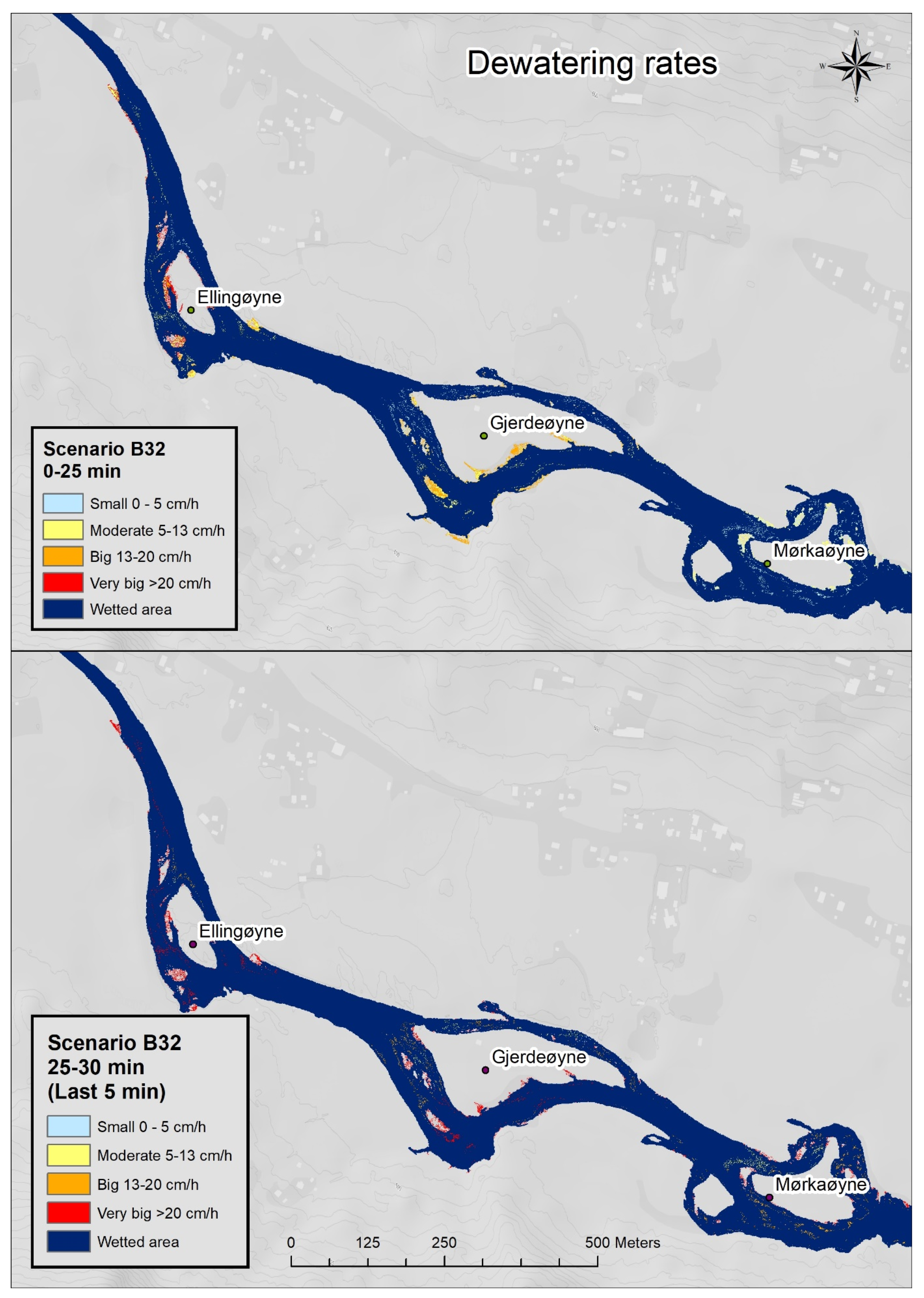B21 consists of decreasing from two turbines to one turbine in 30 minutes, in the first 25 minutes it decreases to 40% of turbine capacity (27 m³/s) and in the last 5 minutes the turbine is completely stopped and only one keeps functioning (21 m³/s). Scenario B32 consists of decreasing from 3 turbines to two turbines in 30 minutes, in the first 25 minutes it decreases to 40% of turbine capacity (42 m³/s) and in the last 5 minutes the turbine is completely stopped and only two keep functioning (36 m³/s). Changing the operation of the turbines will reduce the benefit for the HPP operator. The cost of this mitigation measure has also been estimated.

2.5. Hydraulic Model Set-Up and Calibration

The Hydrologic Engineering Center’s River Analysis System (HEC-RAS 5.0.3.) developed by the U.S. Army Corps of Engineers Institute for Water Resources Hydrologic Engineering Center, 609 Davis, California, USA [29] was used for the hydraulic simulations. The simulations were based on the Diffusion-Wave Form of the Momentum equation [30]. The Manning n was set to 0.06, a value which corresponds” to rivers whose bed is sand and gravel with some boulders and banks with overhanging bushes and trees [31]. Other values were tested (0.03, 0.04 and 0.05) but results differed less than 0.01 m and therefore it was decided to use 0.06 for the entire domain. The input geometry was the DEM with a resolution of 0.5 by 0.5 m. Mesh resolution has a noticeable effect on the computational accuracy of the water-surface elevations and velocities prediction [32]. However, if the grid becomes smaller, the time-step should also be shortened according to the Courant’s condition, with longer computational time as a result. The Courant number or Courant condition is used to ensure stability and accuracy in an unsteady model [30]. When we define a computation time step for our unsteady model, the Courant number has to be smaller or equal 1. Several iterations were made to achieve an optimized grid and time-step that allowed us to carry out the study in a feasible and efficient time frame. Finally, the computational mesh was created with 1 m resolution in mid-stream and 0.25 m resolution along the river banks. This way we could use a higher resolution in areas of interest (river banks where stranding is an issue) and decrease number of points of the model in areas where stranding effect is no issue. The final time-step used was 0.5 s. Boundary conditions were introduced upstream and downstream of the reach. The upstream boundary condition was a flow hydrograph corresponding to the releases from the power plant, and downstream boundary condition was a normal depth with a slope of 0.01 that was measured in the area of the downstream boundary. Still this boundary was set well downstream of the actual study reach. Other values of the downstream slope were tested but the results of the model changed less than 0.01 m.

Calibration was made by using three main data sources covering a discharge from 2.44 to 44.72 m³/s. The sources used were the water edge provided by AHM and computed from the LiDAR data at the time of measurement, a set of RTK-GPS (Real-Time Kinematic Global Positioning System) measurements (Leica Viva CS15, developed by Leica Geosystems Ag, CH-9435 Heerbrugg, Switzerland) of the water edge for four different discharges (Figure 3) and finally aerial pictures from Norge i bilder (www.norgeibiler.no).

The comparison with the water edge from the Lidar survey was made visually as a first approach to check the model performance. We analyzed this with an unsteady simulation with a continuous discharge of 31.72 m³/s, which was the discharge at the day of the flight.

For the GPS-measured water levels, we did simulations with continuous flow for every calibration discharge, imported the computed water surface elevation (WSE) from HEC-RAS into ArcGIS, and then compared this with the measured GPS elevation.

Finally, to obtain a broader range of discharge for comparison we selected an aerial picture from Norge i bilder (www.norgeibilder.no) from 2006 with a recorded discharge of 2.44 m³/s. The picture has a resolution of 0.5 m; therefore, calibration uncertainties are higher, but this resource gave us the opportunity to compare well below any discharge available during the field measurements. The comparison is made visually by contrasting the wetted areas and water edge in the picture with the simulation (see Figure 3).

The HEC-RAS simulations were compared with a total of 253 GPS points measured along the water edge. These points were compared with a simulated water level at the same discharge as at the time of the measurements. The comparison gave a mean error of 6 cm and a standard deviation of 6 cm (Figure 3). It is worth noting that the accuracy of the LiDAR data is 3 cm [28] and the accuracy of the GPS is between 1.5 and 3 cm. Based on this we find the model to be well-calibrated for our purpose.

The comparison with the water edge of the LiDAR survey flight and the aerial picture were very similar to the model simulation for the corresponding discharges (31.72 and 2.44 m³/s) shown in Figure 3. The picture from Norge i bilder was taken with 2.44 m³/s and represents only residual flow coming from the river upstream.

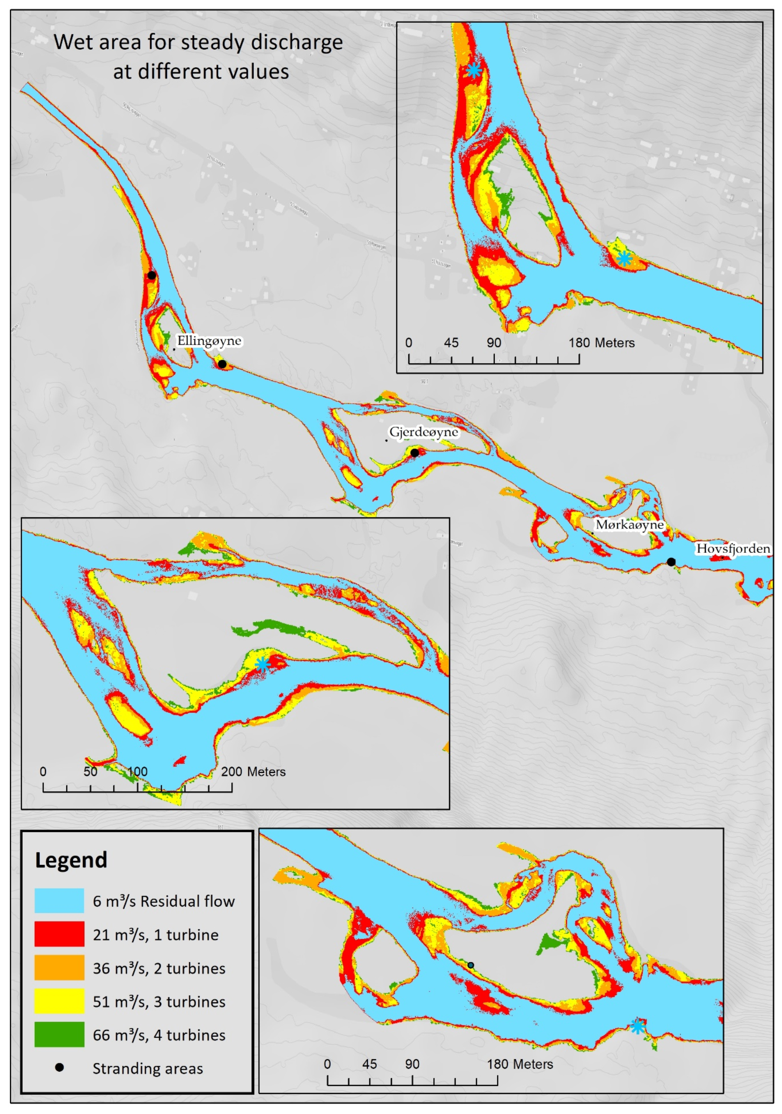
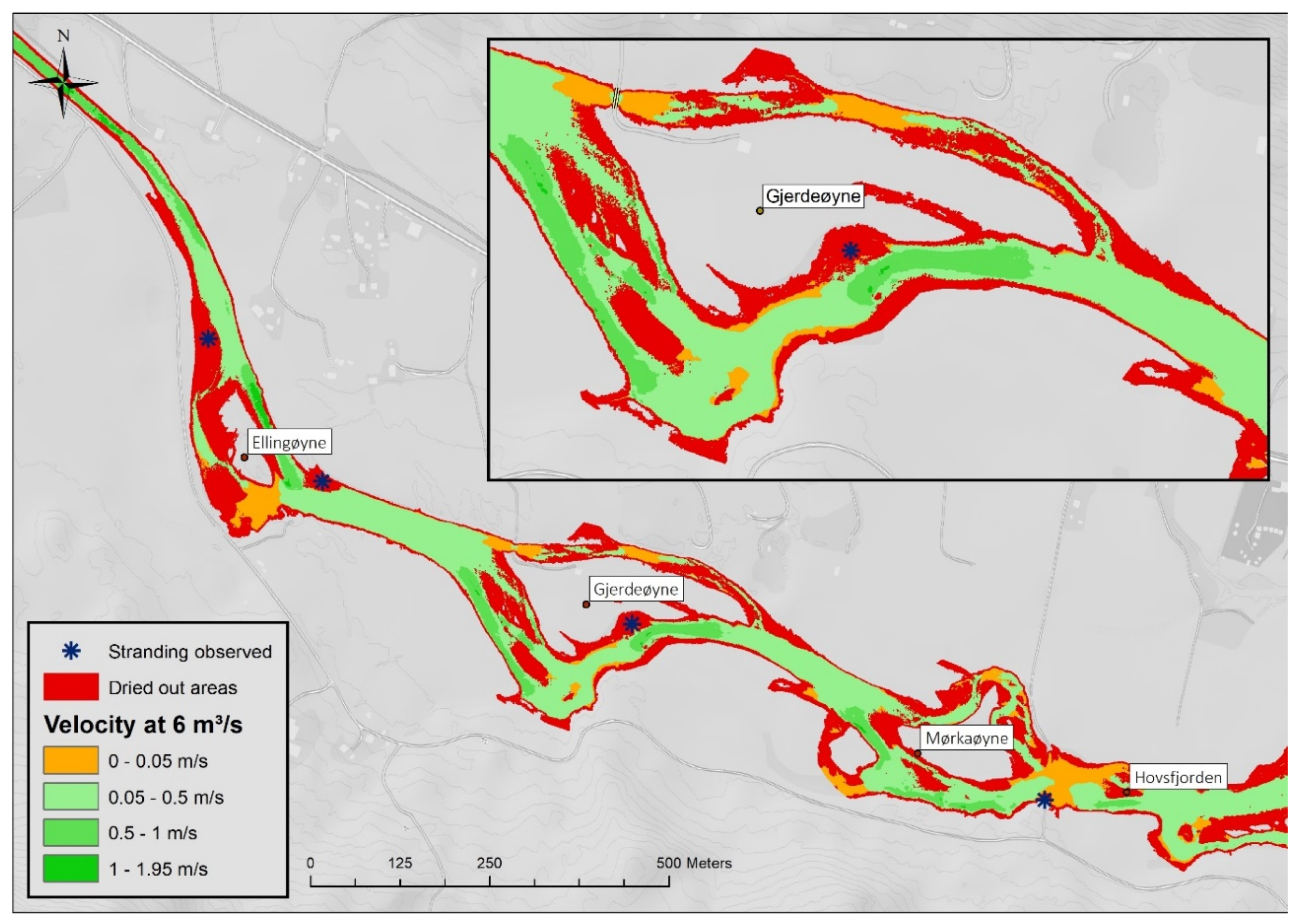
2.5.1. Variation of Wetted Areas

The maximum potential stranding areas are those which dry out when flow is passing from high to low. We simulated all discharges for the different shutdown scenarios and computed the wetted area for each. The dried-out area is then calculated from a reference discharge of 66 m³/s representing full production. These areas are presented as different maps representing dried areas as a function of the number of turbines that are running at the start and at the end of the scenario.

The middle step of scenario B21 with one turbine running at full production and another one at 40% of full capacity (see Figure 2, Scenario B21) is referred as turbine 1.4. Correspondingly, turbine 0.4 represents the middle step of scenario B10, when there is one turbine running at 40% of full capacity.

We also calculate the marginal dried-out area per unit of flow (m³/s). It is calculated as the dried-out area increase divided by the corresponding discharge.

$$\mathrm{Dried}-{\mathrm{out} \mathrm{area}}_{\mathrm{i}} \left(\frac{{\mathrm{m}}^2}{\frac{{\mathrm{m}}^3}{\mathrm{s}}}\right)=\frac{{\mathrm{Dried} \mathrm{area}}_{\mathrm{i}}-{\mathrm{Dried} \mathrm{area}}_{\mathrm{i}-1}}{{\mathrm{Reduced} \mathrm{discharge}}_{\mathrm{i}}},$$

(1)

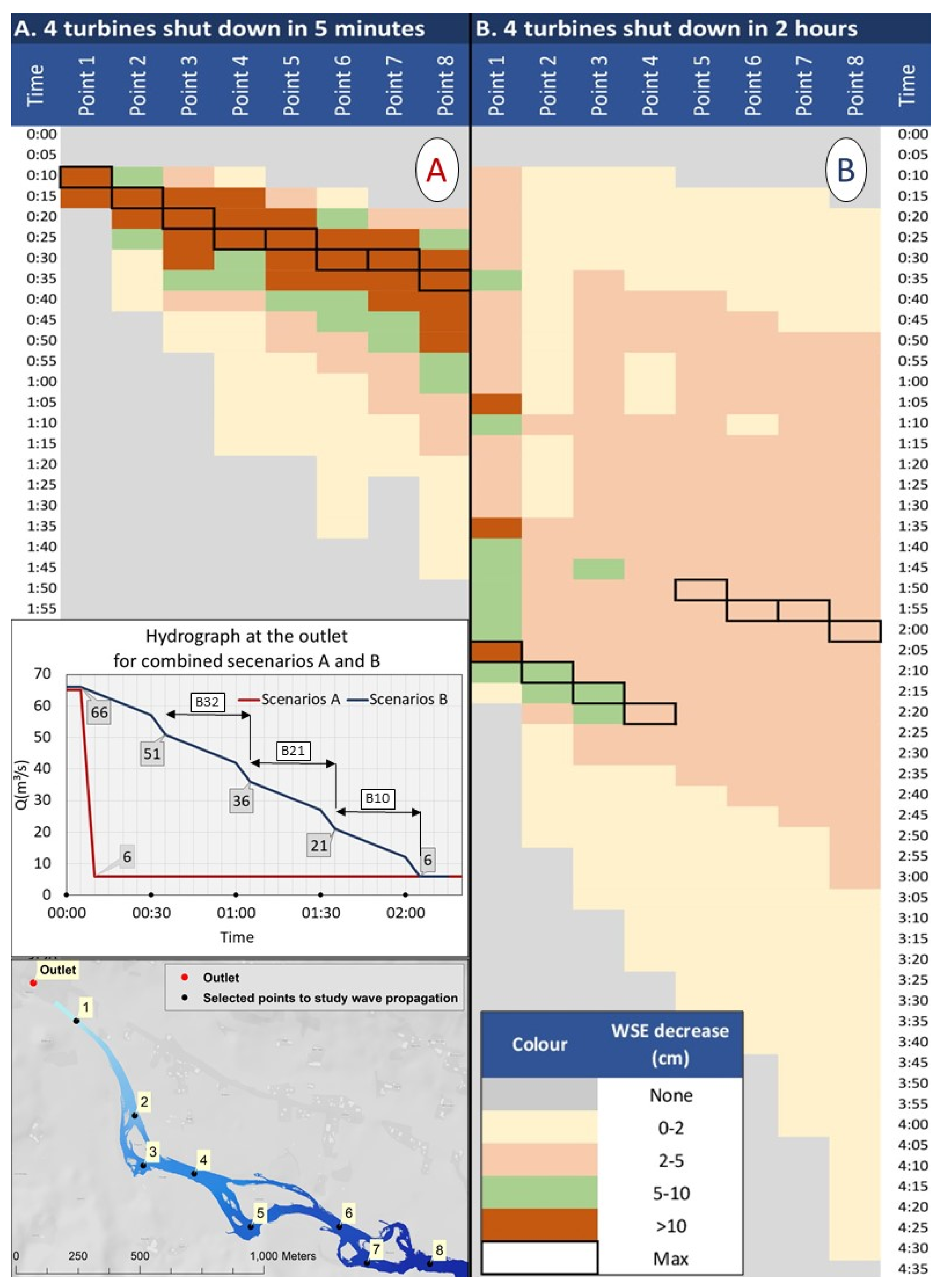
2.5.2. Consideration of Damping Effect in Dewatering Ramping Rate along the Stream

The damping effect is a decrease in the amplitude of an oscillation because of energy being transformed to overcome frictional or other resistive forces. In our case when the turbine is shut down, it creates a wave that will be steep and marked right after the outlet but will become smoothed the further downstream it travels. This factor needs to be considered when calculating the dewatering ramping rate.

A simulation of 3 hours of duration was run to enable the evaluation of the damping effect. In the first 5 minutes the discharge changes from 66 m³/s (four turbines plus residual flow) to 6 m³/s (residual flow).

We generated water surface elevation (WSE) maps every 5 minutes, a total of 35 WSE maps over the duration of the shutdown process. The maps were computed in HEC-RAS and imported into ArcMap for further analysis. From each map we extract WSE from 10 representative points along the river to evaluate the damping effect.

2.5.3. Evaluation of Dewatering Ramping Rate

Stranding of juvenile fish has been a documented consequence below hydropeaking power stations [13]. Ramping rates are important to consider to ensure habitat improvements [33], and according to Halleraker [7] ramping rates higher than 10 cm/h will increase fish stranding risk.

In this study we evaluate the dewatering rate according to the Envipeak guidelines, which define four impact levels according to the dewatering speed: very big, big, moderate and small [5] (see

Table 1. Dewatering velocity rates (with color code) to assess the impact of hydropeaking [5].

Impact	Dewatering Velocity (cm/h)
Very big	>20
Big	13–20
Moderate	5–13
Small	<5

). We define the dewatering ramping rate as the critical velocity rate recorded during an episode with a 5-minute resolution.

The dewatering ramping rate maps for each scenario are created by subtracting the WSE at the end from the WSE at the start of the scenario divided by time. Notice that this time is not the same in every point due to the damping effect and therefore we need a raster map in which every point has a different duration depending on the distance from the outlet.

3. Results

3.1. Characterization of Flow and Rapid Fluctuations

The mean flow downstream Hol 1 hydropower plant is 35.91 m³/s. The minimum flow recorded was 2.38 m³/s on the 6 September 2013 while the maximum flow was 150.08 m³/s on the 6th of September 2011. Notice that the 5-percentile discharge (6 m³/s) and the 95-percentile discharge (64 m³/s) correspond with the minimum and maximum discharges in the modelled scenarios (see

Table 2. Descriptive statistics of flow data from 2010 to 2017 downstream of Hol 1 hydropower plant.

Parameter	Min Flow	5-Percentile	10-Percentile	Mean Flow	90-Percentile	95-Percentile	Max Flow
Discharge (m3/s)	2.38	6.16	8.67	35.91	61.10	64.18	150.8

).

The number of increases and decreases per year has varied among 168 to 331 over the period, but has been over 280 since 2012 as seen in Figure 4. This indicates a river where hydropeaking is frequent.

3.1.1. Discharge Value at Start and End of The Fluctuations

Most of the rapid increases started at relatively high discharges (mean 31.10 m³/s). Correspondingly, most of the rapid decreases stopped at relatively high discharges (mean 29.72 m³/s). However, 25% of fluctuation limits are below 16 m³/s and 10% are below 8 m³/s (

Table 3. Descriptive statistics for the discharge at the start of an increase and the end of a decrease in the period 2010 to 2017 downstream Hol 1 hydropower plant.

Descriptive Statistics	Start	End
2010–2017	Increases	Decreases
Units	m3/s	m3/s
Minimum	2.38	2.95
10th-Percentile	7.77	7.21
25th-Percentil	15.82	15.14
Mean	31.10	29.72
Median	32.03	31.30
75th-Percentil	44.54	42.69
90th-Percentile	53.37	50.68
Maximum	74.78	65.81
Standard dev	16.71	15.79

).

3.1.2. Seasonal Analysis

In Storåne, most of the increases occur during winter (21%) and autumn (24%) in daylight conditions, meanwhile most of the decreases occur during darkness in winter (21%) and autumn (24%). Fewer rapid fluctuations occur during summer (3%) increases in daylight and 14% decreases in darkness) see Figure 5.

3.2. Hydraulic Modelling

3.2.1. Variation of Wetted Area

In the investigated area, our simulations return a wetted area of 140,937 m² under full production conditions against 93,280 m² under residual flow conditions. We consider four turbines in operation plus residual flow (66 m³/s) as a reference for maximum wetted area. When we go from four to three working turbines the area reduction is 5%; from four turbines to two turbines the area is reduced by 15%, with only one turbine working (21 m³/s) the dried-out area is 22% and with no production and residual flow (6 m³/s) the dried-out area reaches 34% (

Table 4. Number of working turbines for different scenarios, its correspondent discharge and reduced discharge, the wetted area associated, dried-out area, percentage of dried-out area and marginal dried-out area per reduced discharge.

Turbine	Discharge (m3/s)	Reduced Discharge (m3/s)	Wetted Area (m2)	Dried-Out Area (m²)	Dried-Out Area (%)	Dried-Out Area (m²)/ Reduced Discharge (m3/s)
4	66	0	140,937	0	0%	0
3	51	15	133,429	7508	5%	501
2,4	42	9	126,411	14,526	10%	780
2	36	6	120,317	20,621	15%	1016
1,4	27	9	112,504	28,433	20%	868
1	21	6	109,316	31,621	22%	531
0,4	12	9	105,173	35,765	25%	460
0	6	6	93,280	47,657	34%	1982

and Figure 6).

The calculations on dried-out area per cubic meter of reduced discharge are shown in Table 4. The table shows that when discharge is between 66 and 51 m³/s a reduction of 1 m³/s will equate to 501 m² of dry area. There is a marked increase in the dried-out area per m³/s reduced flow below a discharge of 12 m³/s, where a reduction of 1 m³/s will equate to a decrease of 1982 m².

Some stream reaches are especially affected at residual flow conditions. The water in the western stream in Ellingøyne is almost completely dried out and stagnant, with velocity below 0.05 m/s (Figure 7), this occurs mainly when flow is lower than 21 m³/s (Figure 6). Stranding fish has been observed in this area (Morten Stickler, personal communication), but this has not been quantified. The southern stream in Gjerdeøyne also has large dry areas at residual flow.

In contrast with Ellingøyne, where the dry areas appear mostly for discharge below 21 m³/s, dry areas in Gjerdeøyne start to appear at discharges below 66 m³/s until residual flow, meaning that this transition is not so abrupt.

The northern and the south-western streams at Mørkaøyne shows big dry areas and also areas with motionless water.

3.2.2. Consideration of Damping Effect in Dewatering Ramping Rate along the Stream

The results show that there is a clear wave attenuation along the stream in Storåne that is quantified by the variation of water surface elevation (WSE). When changing the hydropower flow from 66 to 6 m³/s in 5 minutes, the duration of the wave (time between the start and the end of a change in WSE) will be longer further downstream. Points shown on the map in Figure 8, from 1 to 8 are the representative points selected to study the wave propagation.

The wave propagation can be clearly observed in Figure 8. The heat map displays all WSE change for the representative points at every five minutes during the shutdown. In point 1 the WSE changes from 642.34 m to 640.91 m within 10 minutes producing the sharpest change in minute 15; in point 3, located in Ellingøyne, the WSE changes from 638.63 m to 637.64 m within 45 min, producing the sharpest change in minute 25; in point 5 located in Gjerdeøyne the WSE changes from 637.16 m to 636.22 m in 65 minutes with the sharpest change in minute 30; in point 8 located downstream Mørkaøyne WSE changes from 635.20 m to 634.21 m in 1 hour and 30 minutes with the sharpest change in minute 40.

In contrast, we ran a simulation with the alternative operation procedure, scenarios B43, B32, 321 and B10, shutting down all the turbines in 2 h instead of in 5 min. In Figure 8 we can see that the wave duration is longer. For example, in point 3, the wave passes in 3 h instead of 45 min, in point 5 located in Gjerdeøyne the wave occurs in 3:30 h instead of 1:05 h and in point 8 in Morkaøyne the wave passes in 4:15 h instead of 1:25 h. In point 1, we still find some WSE decrease over 10 cm at 1:10, 1:40 and 2:10, these are the consequence of shutting down from 40% load to full stop in 5 min, which induced a faster dewatering that cannot be mitigated by changing the operation of the turbines.

Results show that the wave critical time depending on distance to the outlet can be approximated by a polynomial trendline with an R² equal to 0.9818. We use this distribution to create a relation between the distance and the time in which the wave occurs for the different scenarios.

3.2.3. Dewatering Ramping Rate

It is clear that Storåne experiences very rapid dewatering at the worst-case scenario with four turbines that are shut down in approximately 5 min. Figure 9 shows the dewatering rate for scenarios A10 and B10 in Ellingøyne. For scenario A10, the whole stream shows dewatering rates over 20 cm/h, considered to be a very big impact in dewatering rate [5]. Notice that the western channel of Ellingøyne (Figure 9) and the northern channel of Gjerdeøyne (Figure A1) will be completely dried-out at a high dewatering rate. The same high dewatering rates occurs for scenarios A21 and A32, and maps can be seen in Figure A1. Areas with observed fish stranding (M. Stickler, personal communication) are also marked on the maps. Six different dewatering scenarios were simulated with 5, 10, 15, 20, 25 and 30 min from full production to shut down. The result shows that for the 25 and 30 min cases, high dewatering impact only affects the artificial channel but not the rest of the river reach.

The alternative scenarios, B32, B21 and B10, with a stop time of 30 min show improvements in the dewatering rate (Figure 9, Figure A2, Figure A3 and Figure A4). For scenario B10 (from 21 m³/s to 6 m³/s) the dewatering impact in Ellingøyne changes from very big to big and moderate, the dewatering impact around Gjerdeøyne changes from very big to moderate and around Mørkeøyne dewatering rate changes from very big to moderate and small. Notice that the further we are from the outlet the lower the dewatering impact due to the natural damping effect of the river (Figure A2).

In the alternative scenarios we also considered the last 5 min in which turbines have to be shut down from 40% capacity to no production (reduction of 6 m³/s in 5 min). This will create fast dewatering rates with big impact in scenarios B, especially for scenario B10 because larger areas are dried out below 21 m³/s (427,794 m²) and two main streams will disappear below 12 m³/s, the western stream in Ellingøyne and the northern stream in Gjerdeøyne (Figure 9, Figure A2, Figure A3 and Figure A4). This is a situation that cannot be avoided by operational constraints.

3.3. Cost of Changing Operation

Changing the operation shutdown from 5 min to 30 min will have a cost for the operator. The calculations on costs are shown in

Table 5. Cost assumptions.

Option	1	2	Units
Estimated price difference	0.1	0.1	NOK/kWh
Spilled water	14,400	14,400	m3/day
Number of decreases	290	87	year
Spilled water	4,608,000	1,382,400	m3/year

and are based on estimated price difference between the maximum price of energy and the price of extra water released.

Two options are presented, option 1 assumes an average number of decreases of 290 per year according to the COSH Tool analysis. Option 2 consists of changing the operation only when the end of the decrease is below 21 m³/s, which occurs for 30% of the decreases, a total of 87 decreases per year. The estimated price difference between the maximum energy price and alternative energy price has been set to 0.1 NOK/kWh (B.O. Dønnum, personal communication). Calculation shows that option 1 would cost 374,587.20 NOK/year ($43,826.70 USD/year) and option 2 would cost 112,376.16 NOK/year ($13,148.20 USD/year) (see

Table 6. Cost calculation for Hol 1 Urunda and Hol 1 Votna.

Group	Hol 1 Urunda	Hol 1 Votna	Units
Energy factor	0.897	1.0017	kWh/m3
Cost Option 1	374,587.20	418,309.92	NOK/year
	43,826.70	48,942.26	US$/year
Cost Option 2	112,376.16	125,492.98	NOK/year
	13,148.20	14,682.68	US$/year

).

4. Discussion

Hydropeaking operations lead to rapid fluctuations in river flow that cause several impacts. These effects can lead to mortality of Atlantic salmon (Salmo salar) and brown trout (Salmo trutta) due to stranding [12,17,34], desiccation or drift of the benthos [6]. However, hydropeaking impact is strongly dependent on river morphology [21,35]. Evaluation of these impacts need high precision geometry like the LiDAR data used in this study, which enables detailed 2D hydraulic modelling for evaluation of these problems. Access to detailed geometry also solves problems with representation of the stranding areas as discussed by [18]. Hydraulic modelling based on existing high-resolution LiDAR data will also improve the decision-making process for developing mitigation measurements in the river.

In this study, we analyzed the rapid flow fluctuations, created a 2D hydraulic model, and evaluated the wetted areas and dewatering rates for different operation scenarios on Storåne River in Hallingdal, Norway. The evaluation was based on the recently available Envipeak guidelines [5].

4.1. Characterization of Flow

The analysis of the time series in Storåne showed that there are over 280 rapid decreases during the year following the pattern of a high impacted hydropeaking rivers [8]. Both the number of rapid decreases and the ratio between the full production and no production (more than 10) are defined as very large by the Envipeak guidelines [5]. The analyses show that 25% of the rapid decreases end at flows below 16 m³/s and 10% below 8 m³/s, which are discharges that will lead to large dry areas, therefore it is highly relevant to quantify these dried-out areas and dewatering rates for low flows to assess the stranding impact in brown trout [7].

The seasonal analysis showed the highest percentage of rapid decreases were during darkness in winter (21%), classified as big impact effect by Envipeak guidelines, and autumn (24%), classified as moderate impact [5]. According to Hedger et al. [17], Sauterleute et al. [36], Scruton et al. [37] and Saltveit et al. [12], a far higher risk of fish stranding occurs during daylight in winter conditions due to the activity pattern of the fish. Therefore, based on our results, dewatering during night might reduce the risk of stranding.

4.2. Performance of 2D Model Based on LiDAR

Airborne LiDAR bathymetry has rapidly evolved in recent years providing high resolution fluvial topography (>20 points/m²) and high accuracy (<10 cm) that has shown to be a good resource for modelling and monitoring meso- and microhabitats by [21]. This report is consistent with our findings, the two-dimensional HEC-RAS model in Storåne was calibrated resulting in a mean error of 6 cm in the z axis, tested for 15 and 45 m³/s.

A previous study shows how one-dimensional hydraulic models have the ability to accurately predict potential stranding areas [18]. But the method presented by Casas-Mulet, et al. [38] still requires a considerable measurement effort to establish the necessary cross sections to reach an accurate representation of the stranding areas.

Combination 1D/2D HEC-RAS model using high spatial resolution (1m) was used to estimate flood hazard area, showing to be an improved tecnique in comparison with the 1D HEC-RAS model [39]. A 2D modelling approach was used in Lundesokna River that allowed a deteailed visualization at any location of the model grid, providing significant information on wetted areas and dewatering velocities [20].

Despite the good performance of the 2D HEC-RAS model, some drawbacks arise. One disadvantage of the 2D model is that it requires substantial computational time and a fine computational grid [39]. LiDAR data is a high resolution technique and very effective to apply in hydraulic models [21], nevertheless we might consider the high initial investment cost that aquiring data with this technology implies. Yet, the cost of acquiring data using LiDAR in a river like Storåne, where the use of sonar is limited would probably be competitive to other methods if the same density of data is required [28]. Finally we can mention that even though the digital topography model has shown to be very accurate, it totally depends on the river morphology scanned by the LiDAR company and changes in river morphology between the years may occur due to floods [21], which would affect the reliability of the model.

4.3. Evaluation of Stranding Areas Based on Two Main Hydro-Morphological Features: Wetted Area and the Dewatering Rate

Dried-out areas appear mostly below 12 m³/s, reaching 34% at 6 m³/s. In the flow range between 6 and 21 m³/s, two main streams will disappear: the western stream in Ellingøyne and the northern stream in Gjerdeøyne. According to the Envipeak guidelines, dry area percentages higher than 20% are considered a very large impact [5]. We also find wider and flatter reaches in Ellingøyne and Gjerdeøyne, this kind of morphology were also found by Tuhtan et al. [19] to have a higher stranding risk. These areas are also near-natural morphology and therefore should be prioritized in terms of mitigation measure compared to artificial habitats [33]. The wetted areas are also an important factor for egg survival, experiments in Lundesokna river have shown that survival rates are lower in areas affected by ramping effects during freezing temperatures [40], which occurs regularly in Storåne during winter. However spawning surveys should be carried to investigate whether this occurs in Storåne.

Hauer et al. [33] stated that longitudinal changes of hydropeaking impacts based on retention processes should be studied further, as there exists an important variation in vertical ramping along the stream. This vertical ramping was particularly higher in the first kilometer downstream of the outlet, which is consistent with our findings. The analysis of the simulations in Storåne show that the damping effect is a key factor to evaluate the dewatering rate. The wave that is produced in 5 min in the outlet (time between start and end of WSE change) will be attenuated reaching one hour and a half at the end of the study site.

The simulation results show that Storåne is highly impacted by hydropeaking. In the current operation procedures, we find large impact in dewatering rate (>20 cm/h) and dry area (>20% from Qmax to Qmin) [5]. Changes in water discharge and water level of this magnitude has been shown to affect behavior in Atlantic salmon [41] and brown trout [7], which could lead to higher mortality during winter.

4.4. Alternative Operation Procedure

Modifications in operational procedures implemented as mitigation measures have been studied by Yin et al. [22] who proposed a method to optimize e-flow and reduce the impacts of dams to help reservoir managers and planners This study shows that a change in the operation can improve stream conditions, reducing stranding risk for brown trout. However, Person [35] showed that implementing operational restrictions like limiting dewatering rates can incur high cost for the power company compared to their ecological effectiveness. With an increasing load of intermittent production in the power grid the demand for balancing services will increase as will the demand for capacity [26] and the effect of alternate operating procedures on the grid stability should be investigated for more than one hydropower station.

On the other hand, Casas-Mulet et al. [38] showed that operational constraints could be devised to mitigate freezing of salmon eggs downstream of a peaking power plant with a relative low cost which mainly related to forced production in periods with sub-optimal power price. The current operation of the Hol 1 power plant show a very big impact in the dewatering rate for all the range of flows according to the Envipeak guidelines [5]. The alternative suggested scenarios (B10, B21 and B32) reduce the impact to moderate and small according to the [5].

The alternative, changing the scenario duration from 5 min to 30 min showed to be the most appropriate according to the dewatering rates. The maps produced show that the dewatering rates in natural areas are below 20 cm/h in the reach when the duration is 25 minutes or higher. As mentioned before, there is a special, high impact when flow is below 21 m³/s; therefore, the first step to reduce impact by operational measures would be changing the shut down time when flow is below this value, meaning that when there is only one turbine working this should be shut down following the scenario B10. It is important to mention that it is possible to decrease the ramping rate between 100% and 40% but the turbines cannot operate at less of 40% capacity, and therefore we must decrease the last 6 m³/s in 5 minutes. This reduction, which probably cannot be avoided by operational constraints, will still have a high impact on dewatering rates on the upstream part of Storåne.

Finally, we calculated the economic cost of the mitigation, $43,826 and $13,148 USD/year depending on the alternative.

As stated earlier there are morphological mitigations to the riverbed that might be carried out to mitigate the impact of hydro peaking. To secure an optimal environmental efficiency in mitigation, both operational and morphological measures should be considered [23,24].

4.5. Transferability of The Method

The method used in this paper can apply to other river where hydropeaking is an issue. The analysis of hydrological time series using COSH-Tool provides an easy way of describing the peaking regime in the river and it allowed for the investigation of both diurnal and seasonal variations [27]. We combined the results of the hydraulic model with guidelines developed in the EnviPeak project [42], which provided an assessment for hydropeaking impact that could be also used in other rivers [5]. This assessment can allow to identify potential stranding areas and critical dewatering rates. The resolution and trustworthiness of the results relies directly on the accuracy of the geometry. We utilized green LiDAR data that provided a high-quality digital elevation model. The cost of LiDAR data is decreasing, and in studies like this it is becoming a competitive technique compared to other data collection methods if the same accuracy in data is needed. However, the method used in this study—including the evaluation of stranding areas and evaluation of the mitigation measure—could be applied to other hydropower systems based on DEMs from other methods like an Acoustic Doppler Current Profiler (ADCP), even if this usually generates a bathymetry with less accuracy than the LiDAR-based method.

4.6. Future Directions

The factors associated with stranding are diverse, when stranding occurs in a given system, the extent of stranding is dictated by the complex interaction of a variety of biotic and abiotic factors [13]. Combination of hydrodynamic and habitat modelling has been used to study stranding and identifying critical discharges [19]. Even if this analysis shows a high impact for the dried areas and dewatering speed, the impacts on the riverine ecosystem can only be assessed in combination with biological data (e.g., fish spawning locations, diversity in invertebrate species) and further abiotic data (e.g., substrate, water temperature).

Substrate is generally very important for brown trout. It can be used as shelter from predators using interstitial spaces [43,44]. According to Bachman, 1984, coarser over finer substrates are important for brown trout. We find this distribution in the area surrounding Ellingøyne and the northern stream of Gjerdeøyne, both with a substrate distribution of more than 45% over 10 cm and low percentage of fines less than 5% [45]. Therefore, we think they would be potential areas to implement habitat measures such as compensation basins, powerhouse outflow deviation or morphological improvements of the river in areas that have been identified as having a high risk of stranding. Mitigating the effects on the river ecology could may also be achieved by altering the river bed morphology and by cutting off some of the high-risk areas; especially those close to the outlet of the hydro power station.

Saltveit and Brabrand [25] carried out a study of fish density at eight different stations along Storåne, three located upstream and five downstream the outlet of Hol 1. The fish density downstream the outlet was shown to be clearly lower than upstream especially among older trout. This could be a consequence of the hydropower operation. Additional data on habitat and fish densities in the river Storåne, both upstream and downstream of the power plant will help in understanding the population effects of hydropeaking. This data will also help in deciding on the most effective mitigation measures in Storåne.

5. Conclusions

This study shows that the two-dimensional HEC-RAS model and a high precision LiDAR dataset combined with the Envipeak guidelines will help to improve the understanding of the current conditions and on the process of mitigating impacts in hydropeaking rivers. The availability of high-precision LiDAR data further strengthened this process. Our results show that under the current operation, Storåne can be highly impacted from the peaking operation. The results show that mitigation is possible to some extent by operational constraints, and a study into the effects of both changing the operational procedures and changing the river bed morphology could be investigated using the models developed for Storåne.

References

1. 2050 Long-Term Stratesgy. Available online: https://ec.europa.eu/clima/policies/strategies/2050_en (accessed on 30 November 2018).
2. Korpås, M.; Trötscher, T.; Völler, S.; Tande, J.O. Balancing of Wind Power Variations Using Norwegian Hydro Power. Wind Eng. 2013, 37, 79–95. [Google Scholar] [CrossRef]
3. Graabak, I.; Jaehnert, S.; Korpås, M.; Mo, B. Norway as a Battery for the Future European Power System—Impacts on the Hydropower System. Energies 2017, 10, 2054. [Google Scholar] [CrossRef]
4. Revision of license terms, NVE. The Norwegian Water Resources an Energy Directorate. In Norwegian, Revisjon av konsesjonsvilkår Norges Vassdrags-og Energidirektorat (NVE). Available online: https://www.nve.no/energiforsyning-og-konsesjon/vannkraft/revisjon-av-konsesjonsvilkar/ (accessed on 23 January 2019).
5. Bakken, T.H.; Forseth, T.; Harby, A.; Alfredsen, K.; Arnekleiv, J.V.; Berg, O.K.; Casas-Mulet, R.; Charmasson, J.; Greimel, F.; Halley, D.; et al. Environmental Impact of Hydropeaking: Knowledge Status and Advice for Government and Industry; NINA Temahefte: Trondheim, Norway, 2016. [Google Scholar]
6. Cushman, R.M. Review of Ecological Effects of Rapidly Varying Flows Downstream from Hydroelectric Facilities. N. Am. J. Fish. Manag. 1985, 5, 330–339. [Google Scholar] [CrossRef] [Green Version]
7. Halleraker, J.H.; Saltveit, S.J.; Harby, A.; Arnekleiv, J.V.; Fjeldstad, H.P.; Kohler, B. Factors influencing stranding of wild juvenile brown trout (Salmo trutta) during rapid and frequent flow decreases in an artificial stream. River Res. Appl. 2003, 19, 589–603. [Google Scholar] [CrossRef]
8. Harby, A.; Halleraker, J. Ecological impacts of hydro peaking in rivers. Int. J. Hydropower Dams 2001, 8, 132–135. [Google Scholar]
9. Lauters, F.; Lavandier, P.; Lim, P.; Sabaton, C.; Belaud, A. Influence of hydropeaking on invertebrates and their relationship with fish feeding habits in a Pyrenean river. Regul. Rivers Res. Manag. 1996, 12, 563–573. [Google Scholar] [CrossRef]
10. Bruno, M.C.; Maiolini, B.; Carolli, M.; Silveri, L. Impact of hydropeaking on hyporheic invertebrates in an Alpine stream (Trentino, Italy). Proc. Ann. De Limnol. Int. J. Limnol. 2009, 45, 157–170. [Google Scholar] [CrossRef] [Green Version]
11. Bejarano, M.D.; Jansson, R.; Nilsson, C. The effects of hydropeaking on riverine plants: A review. Biol. Rev. 2018, 93, 658–673. [Google Scholar] [CrossRef]
12. Saltveit, S.; Halleraker, J.; Arnekleiv, J.; Harby, A. Field experiments on stranding in juvenile Atlantic salmon (Salmo salar) and brown trout (Salmo trutta) during rapid flow decreases caused by hydropeaking. Regul. Rivers Res. Manag. Int. J. Devoted River Res. Manag. 2001, 17, 609–622. [Google Scholar] [CrossRef]
13. Nagrodski, A.; Raby, G.D.; Hasler, C.T.; Taylor, M.K.; Cooke, S.J. Fish stranding in freshwater systems: Sources, consequences, and mitigation. J. Environ. Manag. 2012, 103, 133–141. [Google Scholar] [CrossRef]
14. Vehanen, T.; Bjerke, P.L.; Heggenes, J.; Huusko, A.; Mäki-Petäys, A. Effect of fluctuating flow and temperature on cover type selection and behaviour by juvenile brown trout in artificial flumes. J. Fish Biol. 2000, 56, 923–937. [Google Scholar] [CrossRef]
15. Flodmark, L.; Vøllestad, L.; Forseth, T. Performance of juvenile brown trout exposed to fluctuating water level and temperature. J. Fish Biol. 2004, 65, 460–470. [Google Scholar] [CrossRef]
16. Bradford, M.J. An experimental study of stranding of juvenile salmonids on gravel bars and in sidechannels during rapid flow decreases. Regul. Rivers Res. Manag. Int. J. Devoted River Res. Manag. 1997, 13, 395–401. [Google Scholar] [CrossRef]
17. Hedger, R.D.; Sauterleute, J.; Sundt-Hansen, L.E.; Forseth, T.; Ugedal, O.; Diserud, O.H.; Bakken, T.H. Modelling the effect of hydropeaking-induced stranding mortality on Atlantic salmon population abundance. Ecohydrology 2018, e1960. [Google Scholar] [CrossRef]
18. Casas-Mulet, R.; Alfredsen, K.; Boissy, T.; Sundt, H.; Rüther, N. Performance of a one-dimensional hydraulic model for the calculation of stranding areas in hydropeaking rivers. River Res. Appl. 2015, 31, 143–155. [Google Scholar] [CrossRef]
19. Tuhtan, J.A.; Noack, M.; Wieprecht, S. Estimating stranding risk due to hydropeaking for juvenile European grayling considering river morphology. KSCE J. Civ. Eng. 2012, 16, 197–206. [Google Scholar] [CrossRef]
20. Vanzo, D.; Tancon, M.; Zolezzi, G.; Alfredsen, K.; Siviglia, A. A modeling approach for the quantification of fish stranding risk: The case of Lundesokna River (Norway). In Proceedings of the 11th International Symposium on Ecohydraulics (ISE), Melbourne, Australia, 7–12 February 2016. [Google Scholar]
21. Mandlburger, G.; Hauer, C.; Wieser, M.; Pfeifer, N. Topo-bathymetric LiDAR for monitoring river morphodynamics and instream habitats—A case study at the Pielach River. Remote Sens. 2015, 7, 6160–6195. [Google Scholar] [CrossRef]
22. Yin, X.A.; Yang, Z.F.; Petts, G.E. Optimizing environmental flows below dams. River Res. Appl. 2012, 28, 703–716. [Google Scholar] [CrossRef]
23. Gostner, W.; Lucarelli, C.; Theiner, D.; Kager, A.; Premstaller, G.; Schleiss, A. A Holistic Approach to Reduce Negative Impacts of Hydropeaking. In Dams and Reservoirs under Changing Challenges; Taylor and Francis Group: London, UK, 2011; pp. 857–865. [Google Scholar]
24. Bustos, A.A.; Hedger, R.D.; Fjeldstad, H.P.; Alfredsen, K.; Sundt, H.; Barton, D.N. Modeling the effects of alternative mitigation measures on Atlantic salmon production in a regulated river. Water Resour. Econ. 2017, 17, 32–41. [Google Scholar] [CrossRef]
25. Saltveit, S.; Brabrand, Å. Tetthet av ørret i Storåne i September 2016; E-CO Energi AS: Oslo, Norway, 2016. [Google Scholar]
26. Statnett. System Operations and Market Development Plan 2017–2021; Stattnett SF: Oslo, Norway, 2017. [Google Scholar]
27. Sauterleute, J.F.; Charmasson, J. A computational tool for the characterisation of rapid fluctuations in flow and stage in rivers caused by hydropeaking. Environ. Model. Softw. 2014, 55, 266–278. [Google Scholar] [CrossRef]
28. Alne, I.S. Topo-Bathymetric Lidar for Hydraulic Modeling-Evaluation of Lidar Data from Two Rivers. Master’s Thesis, Norwegian University of Science and Technology, Trondheim, Norway, June 2016. [Google Scholar]
29. The U.S Army Corps of Engineers Hydrologic Engineering Center. HEC-RAS. Available online: http://www.hec.usace.army.mil/software/hec-ras/ (accessed on 23 February 2019).
30. Brunner, G.W. HEC-RAS River Analysis System User’s Manual Version 5.0; US Army Corps of Engineers Institute for Water Resources Hydrologic Engineering Center: Davis, CA, USA, 2016.
31. Barnes, H.H. Roughness Characteristics of Natural Channels; US Government Printing Office: Washington, DC, USA, 1967.
32. Ghamry, H.; Katopodis, C. Computational optimization in simulating velocities and water-surface elevations for habitat–flow functions in low-slope rivers. J. Ecohydraul. 2017, 2, 99–121. [Google Scholar] [CrossRef]
33. Hauer, C.; Holzapfel, P.; Leitner, P.; Graf, W. Longitudinal assessment of hydropeaking impacts on various scales for an improved process understanding and the design of mitigation measures. Sci. Total Environ. 2017, 575, 1503–1514. [Google Scholar] [CrossRef] [PubMed]
34. Hunter, M.A. Hydropower Flow Fluctuations and Salmonids: A Review of the Biological Effects, Mechanical Causes and Options for Mitigation; Department of Fish and Wildlife: Washington, DC, USA, 1992.
35. Person, E. Impact of Hydropeaking on Fish and Their Habitat. Ph.D. Thesis, École polytechnique fédérale de Lausanne EPFL, Lausanne, Switzerland, July 2013. [Google Scholar]
36. Sauterleute, J.F.; Hedger, R.D.; Hauer, C.; Pulg, U.; Skoglund, H.; Sundt-Hansen, L.E.; Bakken, T.H.; Ugedal, O. Modelling the effects of stranding on the Atlantic salmon population in the Dale River, Norway. Sci. Total Environ. 2016, 573, 574–584. [Google Scholar] [CrossRef] [PubMed]
37. Scruton, D.A.; Pennell, C.; Ollerhead, L.M.; Alfredsen, K.; Stickler, M.; Harby, A.; Robertson, M.; Clarke, K.D.; LeDrew, L.J. A synopsis of ‘hydropeaking’studies on the response of juvenile Atlantic salmon to experimental flow alteration. Hydrobiologia 2008, 609, 263. [Google Scholar] [CrossRef]
38. Casas-Mulet, R.; Alfredsen, K.; Killingtveit, Å. Modelling of environmental flow options for optimal Atlantic salmon, Salmo salar, embryo survival during hydropeaking. Fisheries Manag. Ecol. 2014, 21, 480–490. [Google Scholar] [CrossRef]
39. Vozinaki, A.-E.K.; Morianou, G.G.; Alexakis, D.D.; Tsanis, I.K. Comparing 1D and combined 1D/2D hydraulic simulations using high-resolution topographic data: A case study of the Koiliaris basin, Greece. Hydrol. Sci. J. 2017, 62, 642–656. [Google Scholar] [CrossRef]
40. Casas-Mulet, R.; Saltveit, S.J.; Alfredsen, K. The survival of Atlantic salmon (Salmo salar) eggs during dewatering in a river subjected to hydropeaking. River Res. Appl. 2015, 31, 433–446. [Google Scholar] [CrossRef]
41. Puffer, M.; Berg, O.K.; Huusko, A.; Vehanen, T.; Forseth, T.; Einum, S. Seasonal Effects of Hydropeaking on Growth, Energetics and Movement of Juvenile Atlantic Salmon (Salmo Salar). River Res. Appl. 2015, 31, 1101–1108. [Google Scholar] [CrossRef]
42. Bakken, T.H. Centre for Environmental Design of Renewable Energy (CEDREN). Available online: https://www.cedren.no/english/Projects/EnviPEAK (accessed on 15 January 2018).
43. Heggenes, J. Effects of short–term flow fluctuations on displacement of, and habitat use by, brown trout in a small stream. Trans. Am. Fish. Soc. 1988, 117, 336–344. [Google Scholar] [CrossRef]
44. Heggenes, J.; Bagliniere, J.L.; Cunjak, R.A. Spatial niche variability for young Atlantic salmon and brown trout in heterogeneous streams. Ecol. Freshw. Fish 1999, 8, 1–21. [Google Scholar] [CrossRef]
45. Bendixby, L.; Sandem, K. Hol 1 Stolsvatn Power Plant, Graft Report—Fish and Freshwater Organisms; 2012; E-CO Energi: Oslo, Norway; p. 5121810. (In Norwegian) [Google Scholar]
Figure 1. Illustration of Storåne river location in Norway and location of the selected study area from the outlet Hol 1 hydropower plant to Hovsfjorden with the braided channels forming around the three main islands.
Water 11 00201 g001
Figure 2. Dewatering scenarios for stranding risk modelling in Storåne River.
Water 11 00201 g002
Figure 3. Calibration: (a) Comparison with LiDAR water edge recorded the day of the flight (Red) at Q = 31 m3/s, (b) Comparison with Norge i bilder picture at 2.44 m3/s, (c) GPS points calibration.
Water 11 00201 g003
Figure 4. Number of peaking events per year in Hol 1 hydro plant.
Water 11 00201 g004
Figure 5. Percentage of rapid increases (left) and rapid decreases (right) by light conditions and season.
Water 11 00201 g005
Figure 6. Wet area for steady discharge and different values: in blue the wet area at residual flow (6 m3/s); in red the wet area with one turbine running and residual flow (21 m3/s); in orange with two turbines running (36 m3/s); in yellow with three turbines (51 m3/s) and in green full production with four turbines running (66 m3/s).
Water 11 00201 g006
Figure 7. Variation of wetted area downstream Hol 1 hydropower plant: in green the velocity of wetted at residual flow, in red the area dried passing from 51 m3/s to residual flow (6 m3/s).
Water 11 00201 g007
Figure 8. Water surface elevation (WSE) for the 10 selected points along Storåne after a discharge variation from 66 to 6 m3/s in 5 min (left) and 2 h (30 min per turbine) for the alternative operation procedure (right). The black squares indicate when the maximum elevation variation occurs in each specific point.
Water 11 00201 g008
Figure 9. Dewatering rate (cm/h) in scenarios A10 and B10 in Ellingøyne, blue shows the wetted areas at the end of the ramping, the rest of the colors display the impact in the areas that are dried out during the ramping, the white stars show the areas where fish stranding has been observed.
Water 11 00201 g009