Stabilized Formulation for Modeling the Erosion/Deposition Flux of Sediment in Circulation/CFD Models


1
Institute of Applied Mechanics, National Taiwan University, Taipei 106, Taiwan
2
Center for Advanced Study in Theoretical Sciences (CASTS), National Taiwan University, Taipei 106, Taiwan
*
Author to whom correspondence should be addressed.
Water 2019, 11(2), 197; https://doi.org/10.3390/w11020197
Submission received: 4 January 2019
/
Revised: 17 January 2019
/
Accepted: 17 January 2019
/
Published: 24 January 2019
(This article belongs to the Special Issue Applications of Computational Fluid Dynamics for Marine and Offshore Engineering)
Abstract
:In field-scale modeling, when the resuspension of sediment is modeled using a hydrodynamic model, a standard and common approach is to add a resuspension flux as the bottom boundary condition in the transport model. In this study, we show that the way of simply imposing an empirical bottom erosion formula as the flux is actually unrealistic. Its inability to stabilize the sediment concentration can cause excessive suspension fluxes in some extreme cases. Moreover, we present a modified erosion/deposition formula to model the resuspension of sediment. The formulation is based on volume conservation in the presence of erosion/deposition near the bottom. By taking into account the prescribed dry density of the bed material, the proposed formulation is able to produce realistic near-bed concentrations while ensuring model stability. The formulation is then tested in a one-dimensional vertical model and field modeling cases using a three-dimensional coastal circulation model. We show that the modified formulation is particularly important in modeling mud resuspension subject to the large bottom stress, which can be a result of waves or a strong river discharge.
1. Introduction
Sediment transport is an important factor influencing estuarine and coastal environments. Dynamics of sediment budgets tightly interact with hydrological process, morphology, and ecological functions in a wide range of spatial and temporal scales. A proper sediment transport model is valuable in guiding the management of water resources in coastal and estuarine areas while facing alterations due to human activities and climate change. The modeling of suspended sediment transport typically involves a hydrodynamics model and sediment transport model. While hydrodynamics modeling has remarkably progressed recently due to the advancing computation power and techniques, modeling sediment transport remains challenging. From the modeling perspective, sediment processes can simply be divided into two regimes [1]. The first regime is found in the regions with dense concentrations of particles, in which particle-particle interactions are intense, resulting in the dominance of friction and collision. The second regime is found in areas of dilute concentration such that hydrodynamic forcing dominates particle motion. The transport of sediment in the first regime is referred to as bed load while the second regime is suspended load. To deal with sophisticated particle-particle interactions, modeling bed load transport relies on empirical parameterization (e.g., [2]). When particle size is small, such as fine sand, silt, and clay, modeling suspended sediment is analogous to the transport of scalar concentration field, C, in conjunction with settling velocity, [3].
Unlike bed load, which is usually connected to morphodynamics, contexts of suspended load are usually more related to hydrodynamic problems in stratified fluid, such as flow instabilities and turbulence suppression. Therefore, typical field modeling for suspended sediment transport usually disregards the associated morphodynamic change (e.g., [4,5]). The typical governing equation describing the evolution of suspended sediment concentration (SSC) is an advection-diffusion equation, which is written as [3].
where is the velocity field obtained from hydrodynamics calculation, and is the eddy viscosity. Equation (1) is a standard approach widely employed in conjunction with various field-scale hydrodynamics models to describe suspended sediment transport. When coupled with the hydrodynamics model, additional sink or source terms in Equation (1) are required to account for deposition or erosion, respectively. Thus, disregarding any lateral transport and vertical turbulent diffusion, an integral form of mass conservation within the bottommost cell is written as
where indicates the control volume, indicates the surface of the control volume, and represents erosion and <0 represents deposition. For a grid cell with vertical size , a sink/source term to be applied to the bottommost cell can be obtained by reducing Equation (2) to
where the overbar indicates the volume average. With a validated hydrodynamics model, the predictability of Equation (1) relies on the appropriate empirical formulas to parameterize sediment inflow flux from the bottom. A formula used to describe the inflow flux from the bottom is called the pick-up function in the context of sand transport [6] or erosion formula in the context of mud resuspension [7]. It is usually formulated based on laboratory flume studies (e.g., [8,9,10,11]) or in situ flume experiment (e.g., [10,12,13,14,15]) as a function of the difference between the bottom shear stress and the critical shear stress of erosion. The erosion rate is usually described as a power-law [15,16,17] or exponential [8,9,10] relationship with the stress difference for the hard bed or the soft bed erosion, respectively. Up to now, the formulation that has been most widely used is the power law with the number of power = 1, which gives the linear relation between the erosion and stress difference, based on the laboratory results of Ariathurai and Arulanandan [18]. It has been used for suspended sediment transport modeling in conjunction with a number of renowned hydrodynamics models, such as the Regional Ocean Modeling System (ROMS) [4,19,20,21,22,23,24,25,26,27], Unstructured Tidal, Residual, Intertidal Mudflat (UnTRIM) model [28], and Finite Volume Community Ocean Model (FVCOM) [29,30]. It disregards the erosion of the top fluffy mud layer (i.e., soft bed erosion). Moreover, several experimental studies show that the power number for the hard bed erosion ranges from 2 to 6. That is, for the more realistic modeling for the bottom resuspension of sediment, an erosion formula that is more sensitive to the stress difference (i.e., either the exponential law or power law with higher power number) needs to be adopted, e.g., the mud transport module in MIKE21 [31]. However, no matter what types of the erosion formula is employed, implementation must be undertaken with caution. A lack of constraints preventing excessive sediment erosion can result in over-resuspension in the model, particular when the erosion formula is sensitive to the stress difference. This is of critical importance in situations involving wave action or strong river discharge, which can lead to strong bed shear stress and erosion. In such cases, excessive erosion that is overpredicted by the model can result in erroneous predictions of sediment transport.
In fact, the simple addition of empirical sink and source terms to Equation (1) is not representative of the actual cases. It should be noted that the erosion and deposition are also associated with the changes in the depth of the water column. Although this change can be small compared to the total depth, as demonstrated in the present study, it plays a key role in maintaining the magnitude of near-bed SSC below that of the dry density of the bed material. This enables predictions of greater precision and stabilizes the simulations. This study reexamines the mechanisms underlying the erosion and deposition while taking into account the conservation of volume on a moving-grid framework. Our derivation shows that the moving-grid calculations provide a connection to the dry density of the bed. In the case of erosion, this prevents excessive erosion and maintains near-bed SSC at values below those of the prescribed dry density of the bed. Based on the moving-grid formulation, we then present modified sink/source terms for regular fixed-grid calculation. Through numerical testing, we demonstrate that the proposed modified sink/source terms are able to produce realistic near-bed SSC. Without a lengthy discussion related to the physical details of sediment transport, the present study emphasizes the importance of considering changes in the depth of the water column during erosion and deposition. It also presents a modified formulation that guarantees model stability while giving realistic values of SSC.
The rest of this article is organized as follows. In Section 2, mathematical expressions of erosion and deposition are derived, and modified sink and source terms are presented. In Section 3, we perform numerical tests using both moving and fixed grids. Moreover, an example of three-dimensional modeling for San Francisco Bay, USA, is presented. The summary and conclusion are then given in Section 4.
2. Modified Erosion/Deposition Equations Based on Moving-Bottom Formulation
Existing modeling frameworks with fixed grids often lead to discrepancies between the model and actual conditions, in which the depth of water slightly increases with erosion and decreases with deposition. To demonstrate this, we start from the general formulation of the Reynolds transport theorem to describe conservation of sediment mass within a control volume (denoted with ):
where the second integral on the left-hand side (LHS) indicates that the integral is taken with respect to the surface of the control volume, and is the velocity relative to the control surface. Erosion and deposition on the bed lead to a corresponding change in control volume. In the following, we deal with cases of erosion and deposition separately.
2.1. Deposition
Neglecting flow velocities that advect sediment, Equation (4) describing the settling of sediment onto the bed can be rewritten as
where is the moving velocity of the control surface due to deposition. As depicted in Figure 1b, disregarding any vertical flux at the top boundary of the control volume, temporal discretization of Equation (5) using the explicit Euler scheme for a control volume of height leads to
where C is the volume-averaged concentration, is the concentration at the bottom boundary, the superscript n represents the computational time step, is the (positive) height of deposition from time = t to , and is the (positive) moving speed of the bottom of the control volume. Treating the bottommost grid cell in the computation domain as the control volume of Equation (6), the concentration within the bottommost cell, denoted as , can be obtained by rearranging Equation (6) as
The third term on the LHS of Equation (6) is the total mass of deposition. Given that the bed material has a dry density, , the height of deposition, , is thereby expressed as . Using the identity, , can be obtained with
Equation (7) describes the “realistic” volume-averaged concentration resulting from only deposition in the bottommost cell, within which conservation of volume is regarded. If is sufficiently small to be disregarded, Equation (7) is reduced to the standard discretized equation on fixed grids to obtain the concentration in the bottommost cell, denoted using the overhat, as
In numerical calculations, is usually extrapolated from interior values, and, in most cases, . Therefore, Equation (10) indicates that, in the case of pure deposition, as long as the deposition height does not exceed height of the cell, the realistic concentration must be less than the calculated value obtained using the standard deposition formula (Equation (9), as depicted in Figure 1a).
2.2. Erosion
The case of erosion differs slightly from that of deposition. One can see this by starting from the general formulation of mass conservation for pure erosion, which is expressed as
where parameterizes a fluctuation velocity that results in the suspension flux of bed sediment into the water column. Due to the fact that complex processes involved in bottom erosion cannot be resolved in any field-scale hydrodynamics model, the second term on the LHS of Equation (11) relies on empirical formulas based on laboratory or field measurements. Practically, the measured mass flux, as denoted by , represents the magnitude of the second integral of Equation (11) (i.e., the net mass flux). Using the same time discretization as in Section 2.1 and disregarding any flux on the top of the control volume, as depicted in Figure 1d, one obtains , where is the (positive) erosion depth and can be obtained with
Again, the volume-averaged concentration in the bottommost cell (denoted as ) can be obtained with
It can be seen that, if is negligible, Equation (13) is reduced to the standard erosion equation describing changes in concentration due to erosion in the bottommost grid cell, i.e.,
Substitution of Equation (14) into Equation (13) leads to
which shows that, with the occurrence of erosion, the resulting near-bottom concentration is always less than the value obtained using the standard erosion formulation (Equation (14)). Although can be sufficiently small so that the difference between Equations (14) and (15) is negligible, the most important feature of Equation (15) is the fact that considering the depth of erosion provides a linkage between the near-bottom concentration () and the dry density of the bed (). One can see this by rearranging Equation (15) to become
Therefore, as is always higher than , Equation (16) shows that concentration in the bottommost cell would never exceed the concentration of the bed material. However, this cannot be guaranteed in the standard fixed-grid implementation (Equation (14)), as depicted in Figure 1c, in which the connection to bed properties is missing. As a result, the boundary condition of bottom erosion is ill-posed in the sense that it can continuously provide sediment through the bottom boundary regardless of the near-bed concentration. This situation can be far worse when power-law or exponential-law empirical formulas are adopted for the parameterization of erosion due to the nonlinear growth of the eroded quantity with the increasing excessive bottom shear stress (e.g., Equation (21)).
In the conditions of strong turbulent mixing, such as strong tidal flows, the resulting stability issue may not be severe because eroded sediments can be soon suspended into the water column and vertically well mixed, but it would not be so when wave forcing is involved. The bottom shear stress resulting from the wave-induced oscillating boundary layer is usually much stronger than those induced by tidal currents only. Moreover, in shallow water estuaries, the wave effect is relatively strong when water depth is low, such as low tides, during which the turbulence intensity is weak. As a result, once eroded, sediments can accumulate in the bottommost cell and exceed the dry density of the bed. When this occurs, the resulting strong buoyant flux of sediment can result in numerical instability and inaccuracy.
2.3. Modified Erosion/Deposition Formula
Based on the previous derivation, we propose the “modified flux” (denoted with the superscript ) to reformulate the bottom sink/source term (Equation (3)) on fixed grids as
in which is derived in accordance with changes in the control volume (Equations (7) and (13)), to obtain
where is the bed shear stress based on hydrodynamic calculation, is the critical shear stress for deposition, and () is the critical shear stress for erosion. In Equation (18), and are calculated using Equations (8) and (12), respectively. It should be noted that Equation (17) does not conserve mass at the water-bottom interface but rather maintains a stable, realistic concentration in near-bed regions. Therefore, if the calculation of deposited or eroded mass is necessary in the cases requiring the estimation of the erosion/deposition depth, the actual eroded mass flux is and deposited mass flux is .
3. Numerical Tests
3.1. 1DV Model
In this section, we conduct simple numerical tests showing the differences among standard erosion formulation, the moving-grid case, and the modified erosion formulation. Because the present study focuses on vertical suspension and deposition, we solve one-dimensional vertical (1DV) equations disregarding any lateral transport. In conjunction with a turbulence closure model, the resulting formulation provides a standard approach to obtain the vertical distribution of SSC in horizontally homogeneous turbulent flow. When taking into account changes in water depth due to erosion and deposition, the 1DV model is solved on the moving frame, with a moving-grid velocity, . Thus, the equations for horizontal momentum (u) and sediment concentration (C) are respectively written as
and
where is the kinematic viscosity of water, is the eddy viscosity, p is the pressure, x is the horizontal coordinate, and is the turbulent Schmidt number. The model is employed for the turbulence closure that also takes the buoyancy effect due to suspended sediments into account [32]. In Equation (19) through Equation (20), is non-zero only in the moving-grid calculation. In that case, the domain depth varies at each time step according to Equations (8) and (12), and new equal-spacing grid cells are obtained accordingly using the same total grid number. Using finite-volume discretization in space, the resulting numerical scheme is an arbitrary Lagrangian Eulerian (ALE) scheme capable of guaranteeing mass conservation [33], representing a simplified version of three-dimensional flow modeling coupled with the moving bed form in Chou and Fringer [34]. As previously mentioned, source and sink terms are added to the bottommost cell of sediment concentration calculation. Here, we use the formulation proposed by Parchure and Mehta [8] for erosion, which is expressed as
where is the erodibility, is the bottom shear stress, is the critical shear stress of erosion, and and are two site-specific constant coefficients. For deposition, we set in Equation (18), i.e., sediments begin to deposit where there is no erosion. According to the field case of cohesive sediment modeling by Lumborg and Pejrup [35] and the values suggested in MIKE 21 [31], this study uses g m−2 s−1, , , and N m−2, which represents erosion over the soft mud layer. Although the choice of these values is arbitrary, it does not affect the conclusions of the present study. Just beneath the water column is a partially-consolidated mud layer with g L−1. In Equation (21), is the result of combined wave current forces. Assuming that the wave orbital velocity is aligned with the current velocity, can be written as [36]
where is the shear stress induced by currents, is induced by waves, and is the angle between currents and waves and is set to 1 here in the 1DV model. In coastal circulation models, can be obtained using the log law with a prescribed value for bottom roughness (), and is calculated based on wave properties that can be obtained through the coupled wave model (e.g., [19]). Thus, is written as
where is the wave friction coefficient and is the wave orbital velocity.
In many cases, can be much higher than such that waves become the major contributor to sediment erosion. However, further suspension into the water column depends on turbulence induced by tidal currents. Therefore, it can be expected that the most unstable case would occur during strong wave events when tidal currents are weak (e.g., during low-water slack tide). Here, for the sake of simplicity, we assigned arbitrary values directly to rather than considering wave properties.
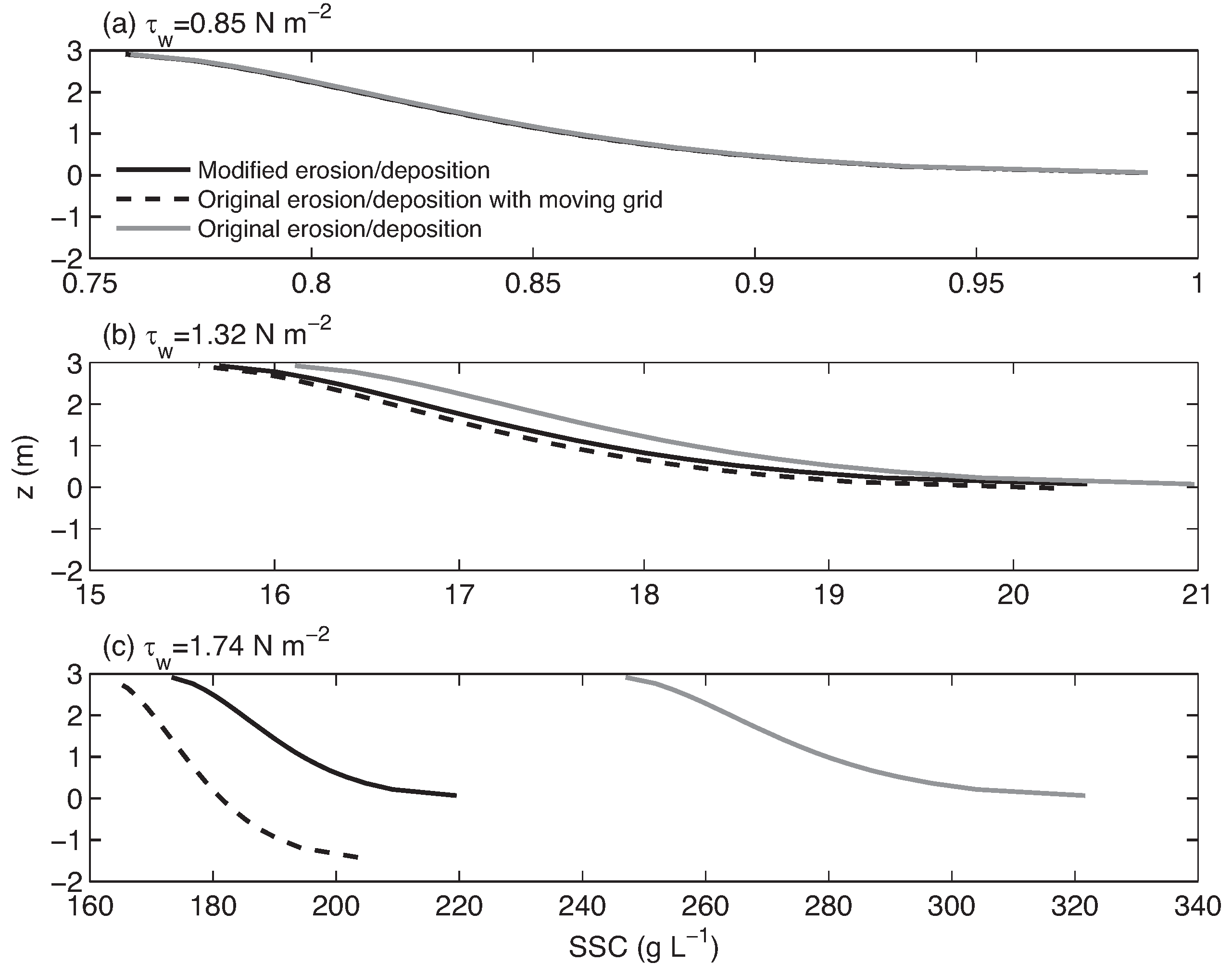
Numerical simulations are performed in a one-dimensional vertical domain with depth of 3 m, discretized using 20 equally-spaced grid cells. A settling velocity of m s−1 is used corresponding to the particle diameter µm based on the Stokes law. A steady current is forced by a pressure gradient resulting in a depth-averaged steady current velocity = 0.2 m s−1. Using the log law with , the simulated is equal to N m−2, which is less than and would not induce any suspension. Three cases associated with different wave conditions are simulated using , 0.70, and 0.82 m s−1. Assuming that the wave period is 10 s and the wavelength is 30 m, thtese s correspond to wave heights of 1.17, 1.49, and 1.75 m, respectively. Using the formulation for given in Madsen et al. [37], these three cases correspond to , 1.33, and 1.74 N m−2. For each wave condition, simulations are conducted according to various modeling approaches. The first is the moving-grid simulation using the original deposition/erosion formulation (Equation (2)). Because it strictly conserves volume, it gives the most realistic and accurate SSC results. Both the second and third modeling approaches are performed on fixed grids. In the second case, we apply the modified deposition/erosion formulation (Equations (17) and (18)). In the third case, the standard approach that directly employs the original deposition/erosion formulation is applied. Sediment erosion begins after the current reaches a steady state, during which eddy viscosity is of a parabolic shape. Simulations are then performed for a three-hour duration, which gives a significant change in depth due to erosion in the case of the strongest wave.
Figure 2 presents results of different modeling approaches for the bottom sink/source terms in different wave conditions. In the case of m s−1 (Figure 2a), the wave-induced shear stress is relatively weak and different modeling approaches give almost the same results. As increases, the difference among cases using different approaches becomes visible, as shown in Figure 2b. In the case when the wave-induced stress is the largest, as shown in Figure 2c, a significant overestimate of SSC can be found using the original erosion/deposition formula. Figure 2c also shows that the modified erosion/deposition formula greatly eliminates the overestimates, which demonstrates the importance of applying the modified erosion/deposition formula when suspended sediment modeling is conducted on the fixed-grid framework. Only little differences are found between cases of the original erosion/deposition formula on moving grid and of the modified erosion/deposition formula, which is due to the difference of the bed shear stresses induced by changing depth in the moving-grid case. Comparison of SSC profiles in different wave conditions in Figure 2 shows that SSC profiles dramatically increase as increases. This is due to the exponential formula (Equation (21)) employed for bed erosion, which is potentially ill posed when applied to the strong wave case on fixed grids without the present modified erosion/deposition formula.
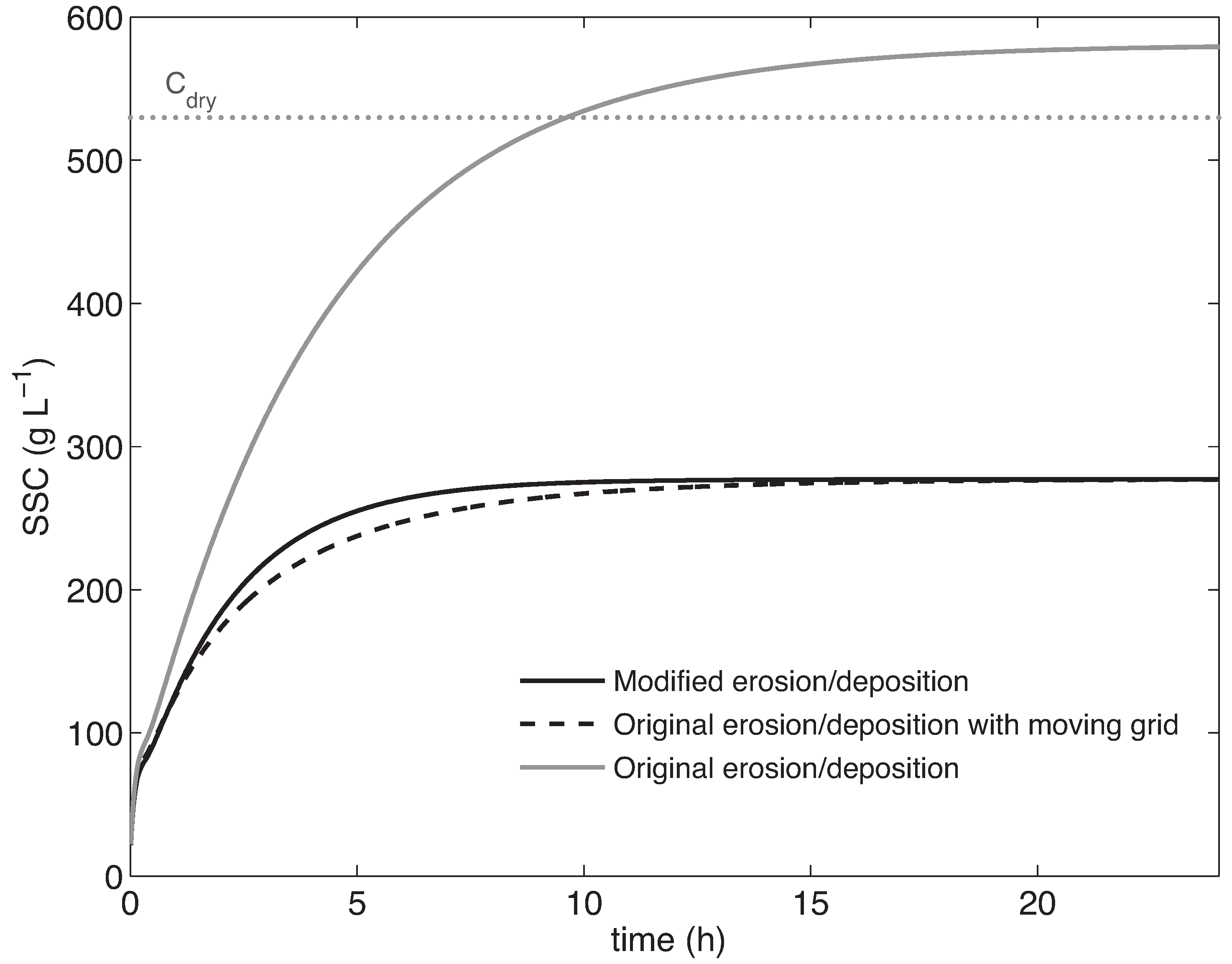
A further run with the strongest is then conducted so that simulations reach the steady state. Although it is not a realistic situation that the critical shear stress remains the same when the bed is being eroded (i.e., the depth-varying should be considered due to mud consolidation), the objective is to examine the potential difference among different modeling approaches in a long-time run using a simple model setting. Figure 3 presents the time series of SSC in the bottommost cell from time = 0 to 24 h, which is the time when all simulated SSCs almost reach the steady state. It can be seen that both the moving-grid and the modified erosion/deposition cases nearly reaches a steady state at time = 10 h, while the case of the original erosion/deposition formulation with fixed grids reach a steady state at time = 24 h. The growth rate of SSC in the case of the original erosion/deposition formulation is faster than the other two cases throughout the simulation, and without any connection to the properties of the bed material in the original erosion/deposition formulation, SSC in the fixed grid simulation exceeds the prescribed dry density (530 g L−1 here) at approximately 10 h.
In this section, we show that, for a simple 1DV model, slight changes in the wave condition may dramatically increase the quantity of eroded sediment. In such a case, implementation of the original erosion/deposition formula disregarding the change in depth can lead to unrealistically high SSC in the modeling result due to the ill-posedness when applying the exponential law to model erosion. Moreover, we demonstrate that, on the non-moving grid, this issue can be fixed by applying the present modified formula, which is able to give SSC results similar to those with moving grids. Therefore, when suspended sediment transport modeling is incorporated with the fixed-grid circulation model, it is recommended to apply the present modified erosion/deposition formula to obtain the stabilized SSC. In the next section, an example of field modeling is presented.
3.2. Three-Dimensional Sediment Transport Modeling of San Francisco Bay, California, USA
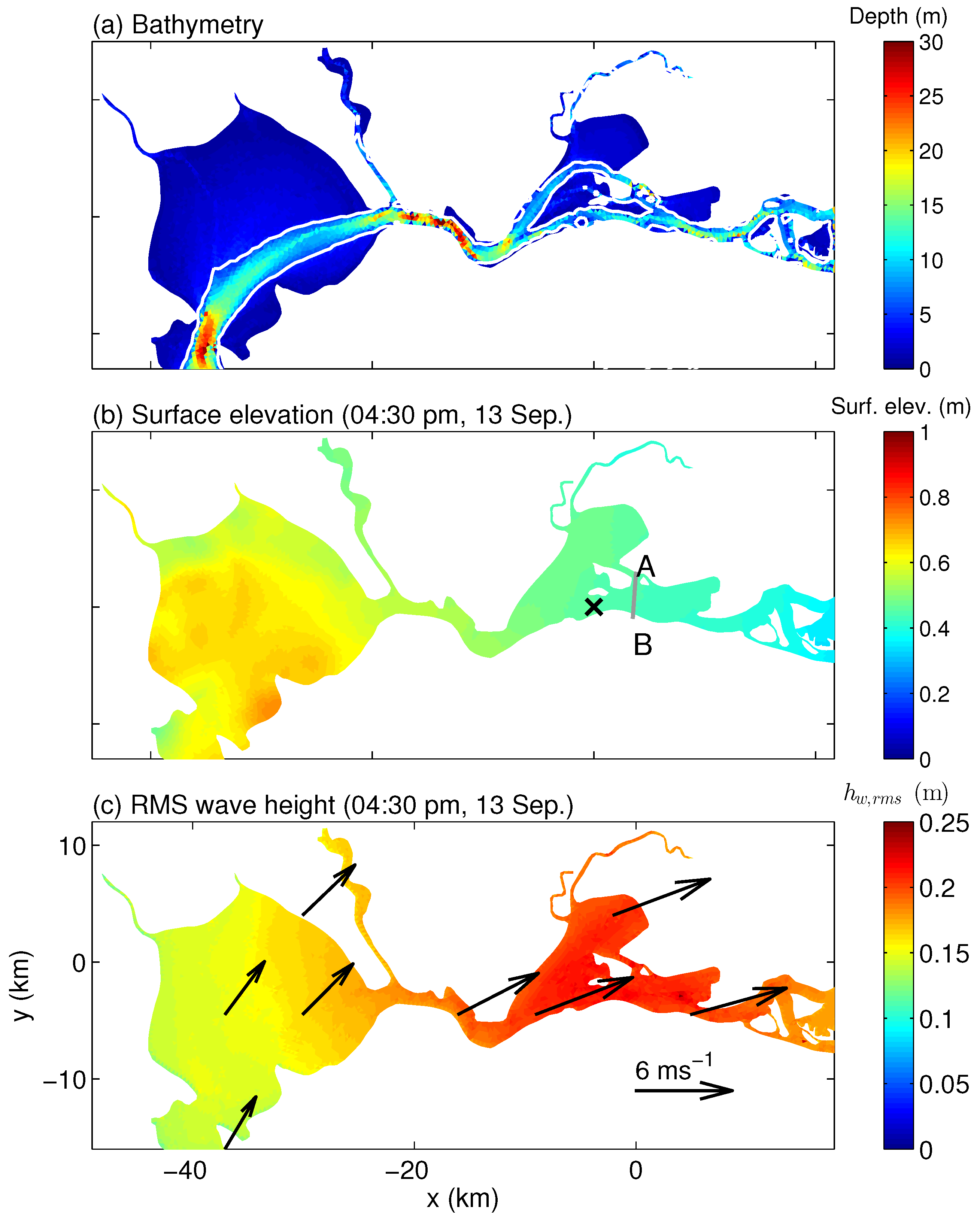
In the second example, we present three-dimensional (3D) modeling of hydrodynamics and sediment transport in San Francisco Bay using the Stanford unstructured coastal hydrodynamics model, SUNTANS. In San Francisco Bay, a distinct channel extends throughout the bay along its thalweg and incises shallow shoals (see Figure 4a). This results in the intriguing dynamics of sediment transport subject to combined wave and tidal forcing, which has been extensively studied in past few decades (e.g., [28,38,39,40,41]). Here, we focus on the comparison of modeled SSC between the conventional and present modified formulation at North San Francisco Bay (North Bay) (i.e., San Pablo Bay and Suisun Bay, see Figure 5) using the validated SUNTANS model, with an emphasis on the consequence of wave forcing. The domain setup of Chua and Fringer [42], who studied tidally driven salinity in San Francisco Bay during January of 2005, is employed here. The same setup was also employed to study hydrodynamics due to waves and tidal currents at South San Francisco Bay during September of 2009 by Chou et al. [43] and the sediment transport by Chou et al. [5]. All these studies showed good agreement compared to field observations. More details of the model and simulation setup can be found in these studies. As we focus on the effect of the modified formulation for modeling erosion and deposition, in what follows, only setup conditions that are relevant to the present results are addressed.
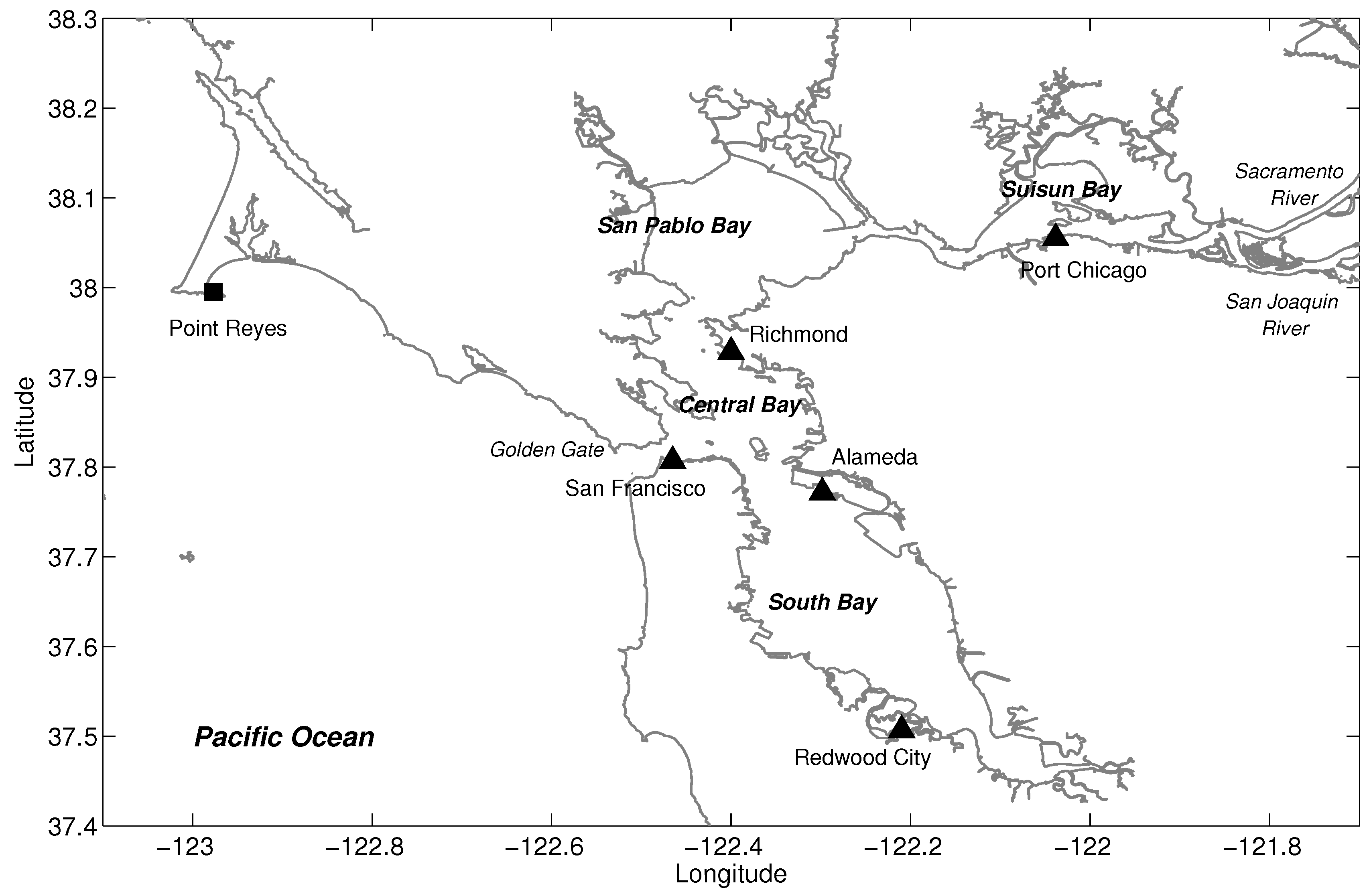
The computational domain spans between the Pacific Ocean and the Sacramento-San Joaquin River Delta, as shown in Figure 5. Open boundaries are at the Pacific Ocean, Sacramento River, and San Joaquin River. The average grid resolution based on triangular cell lengths is 50 m. In the vertical, the z leveled grid has a maximum of 60 layers in the deepest portion of the domain. The vertical resolution is refined near the surface with a grid stretching ratio of 10%, resulting in a minimum vertical grid spacing of 0.29 m. The total number of cells in the horizontal is approximately 80,000. The flow is forced by specifying free-surface elevation along the Pacific Ocean boundary using the data at Point Reyes (see Figure 5), which is obtained from the National Oceanic and Atmospheric Administration (NOAA) Center of Operational Oceanographic Products. Flow rates at the Sacramento and San Joaquin Rivers are given by freshwater inflow estimates from the DAYFLOW program of the California Department of Water Resources. A time step of 10 s is employed to ensure stable horizontal advection of scalars. Waves are generated due to winds, and their transport is modeled using the wave-action approach following Booij et al. [44] on the same grid with the same time step as the hydrodynamics model. Wind speed and direction are reconstructed as each grid cell by interpolating wind data from five NOAA wind stations, as shown in Figure 5. More details of the wave model and simulation setup can be found in Chou et al. [43]. For the sediment transport model, according to the field study by Manning and Schoellhamer [45], two size classes are used to model a slowly- and fast-settling components, respectively. For the bed, a multi-layer bed sediment model [5] is used. In this model, the bed is vertically divided into three layers, and each layer is assigned with different erodibility (), critical shear stress for erosion () (see Equation (18)), height , and dry density . Moreover, consolidation rates are assigned to act as a mass exchange between bed layers. More details of the bed model can be found in Chou et al. [5]. Properties of the bed sediment are summarized in Table 1. Resuspension of the bed sediment into the water column is modeled in the way that once the bottom stress exceeds the critical shear stress for erosion, quantities of resuspended sediment are calculated by Equation (21) and divided into each size class according to prescribed fractions. The fraction of each size class, as denoted by (j in the class index), is empirical and needs to be calibrated with the field measurement. According to Chou et al. [5], with (fine) and mm s−1 (coarse), = 5% ( = 95%) in regions where the depth < 5 m and = 30% ( = 70%) in regions where the depth ≥ 5 m give the best agreement with the field data. Here, following previous studies, we use these setup conditions with the original and modified resupension formulas for comparison.
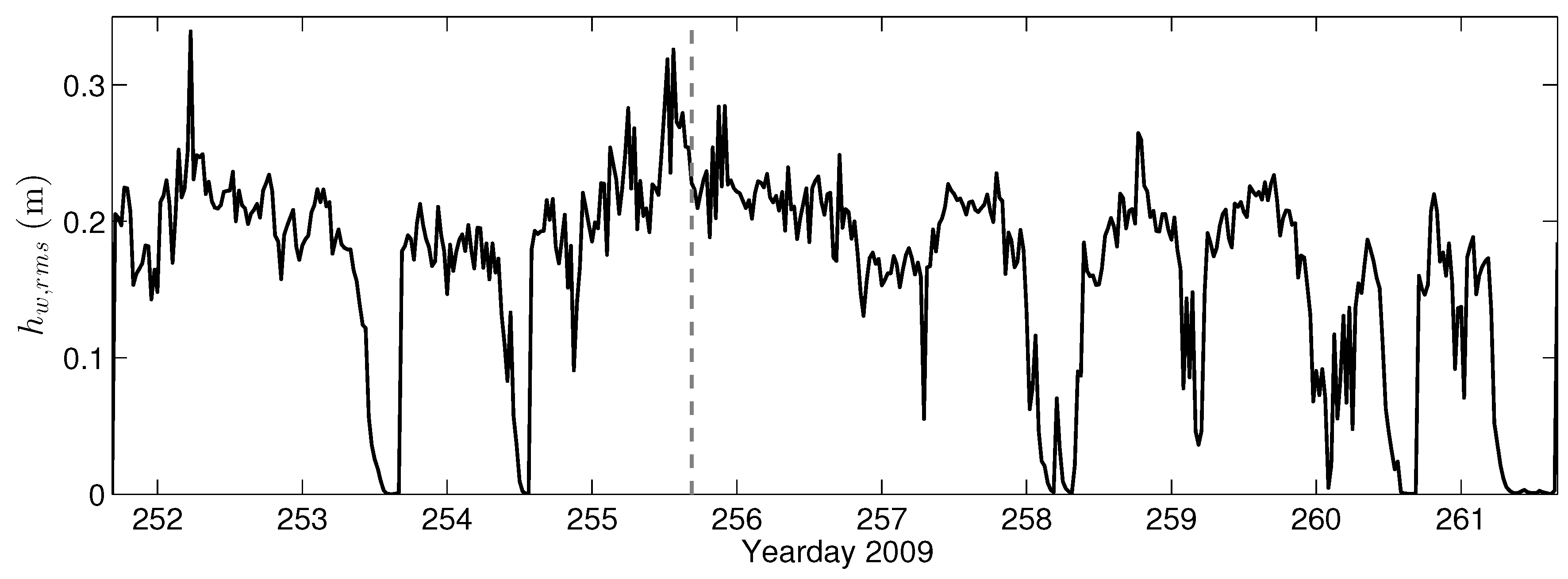
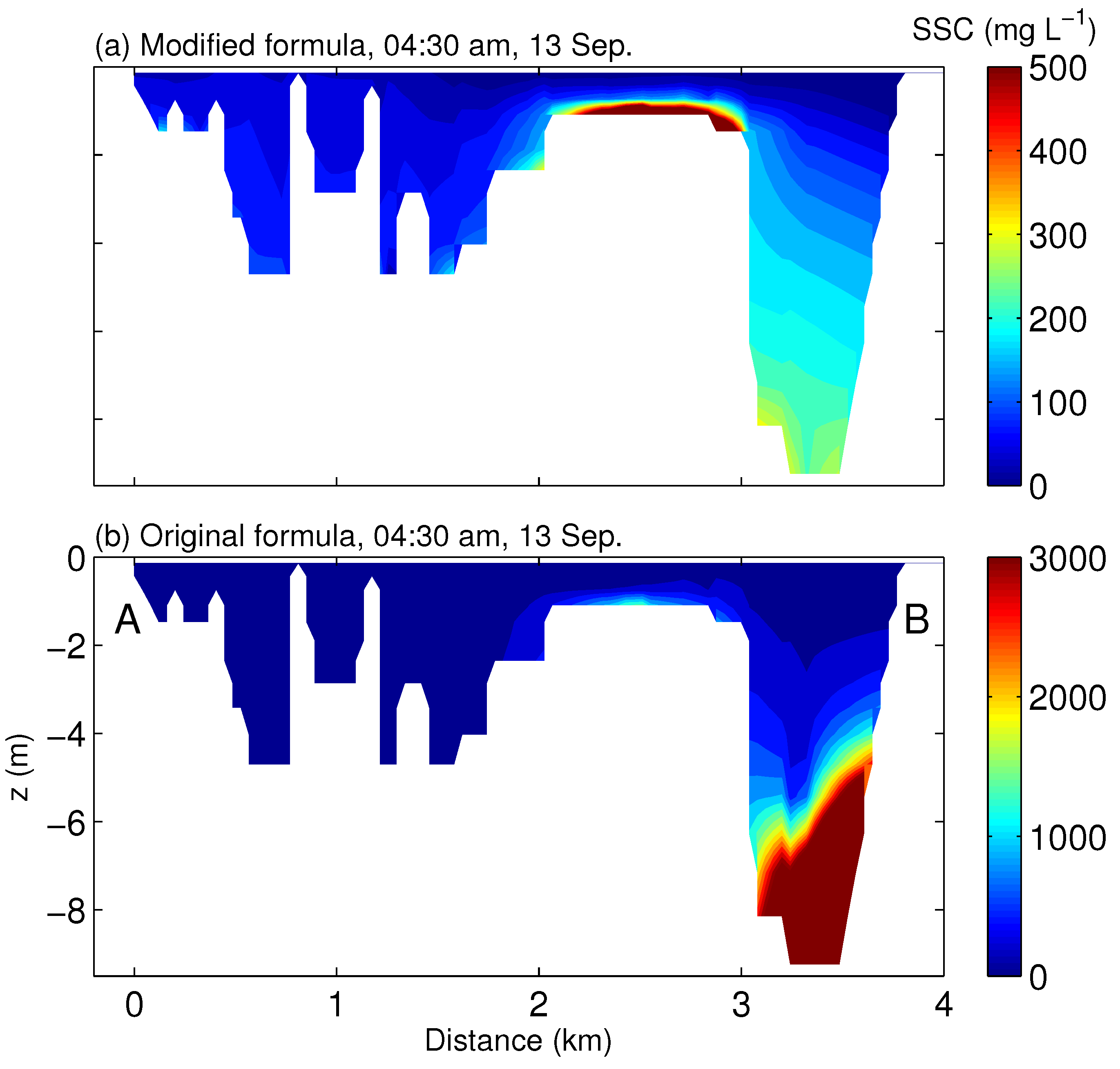
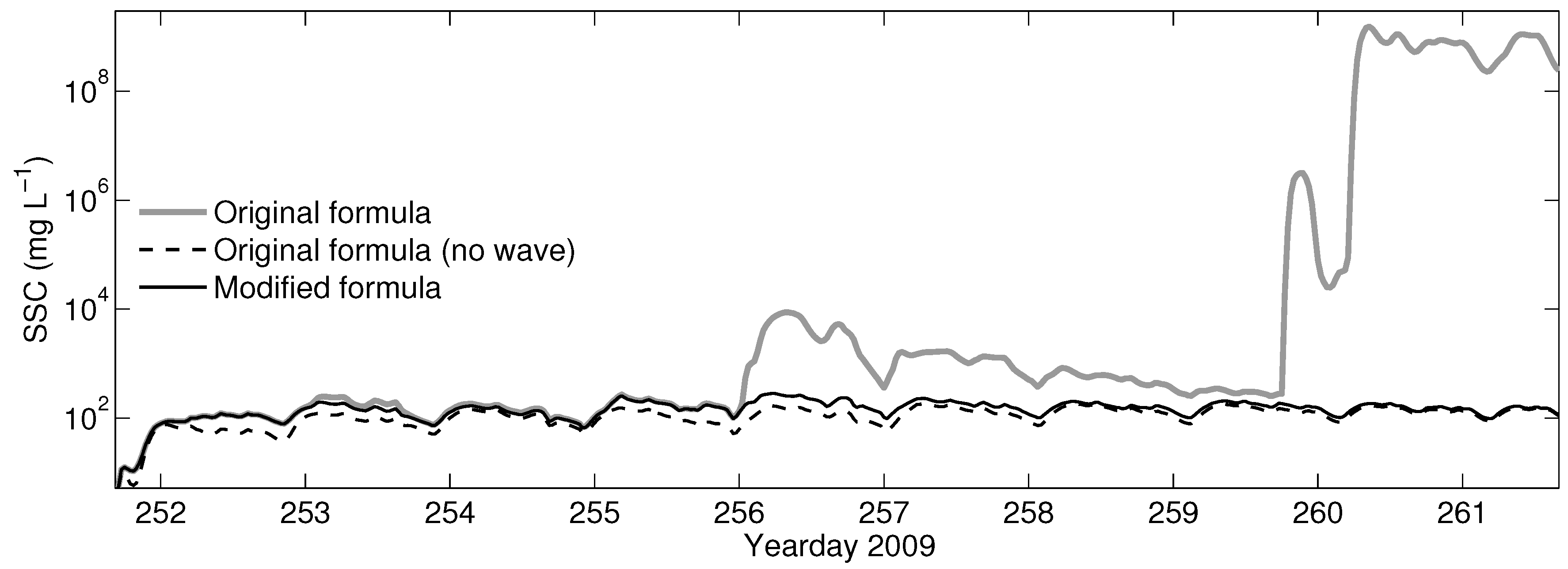
Figure 6 presents the time series of the root mean squared (RMS) wave height, , measured near the Port Chicago wind station, as indicated by the cross in Figure 4b. During the summer, winds coming from the Pacific Ocean result in persistent wave events in the Bay. As shown in Figure 6, the wave event persists during yeardays 255–256. Here, we choose the time point of 4:30 p.m. on the yearday 255 (13 September 2009) for the following discussion. This time point is chosen also because it is the time when SSC predicted by the original resuspension formula starts to deviate from those by the modified formula and becomes unrealistic. The corresponding surface elevation and the resulting distribution of the RMS wave height along with the wind field are shown in Figure 4b,c, respectively. During the time, as shown in Figure 4c, modeled waves are relatively strong at the Suisun Bay without significant breaking, which results in strong near-bottom orbital velocities. As shown by the transect in Figure 7a, particularly in regions of low water depth, this leads to high near-bottom SSC, which can further transport into the deep-water channel [5]. However, without modification, the exponential relationship given by Equation (21) can easily lead to extremely high sediment concentration near the bottom, which subsequently makes the SSC in the water column unrealistically high, as shown in Figure 7b. A comparison between Figure 7a,b clearly shows that the modeled near-bed SSC can be stabilized by the present modification. The temporal evolution of the horizontal distribution of the near-surface SSC in the case with the original resuspension formulation is presented in Figure 8. It can be seen that the modeled SSC begins to grow significantly and forms certain spots of the high concentration (see Figure 8a,b). The subsequent dramatic growth during the persistent wave events results in unrealistically high SSC in the channel (see Figure 8c,d), which can be eliminated by applying the present modification for the suspension formula. Figure 9 shows comparison of time histories of the point measurement for the near-surface SSC between cases with modified and original resuspension formulas, along with the case without the wave effect. First, compared with the case without waves, Figure 9 shows that considering the wave effect (with the modified formula) significantly enhances SSC in the water column, indicating the dominance of waves in resuspending bed sediment. In the present case, the strongest wave effect in the case with the modified formulation almost doubles the SSC compared with the case without waves (during yeardays 256–257). Moreover, without any stabilizing effect for the resuspension formula, Figure 9 also shows an unrealistic growth in SSC after the yearday 256, which demonstrates the importance of the present modification when modeling the wave-induced resuspension.
In fact, it should be noted that a more detailed field survey for the realistic bed properties, such as the erodibility as a function of the erosion depth, may also prevent the unstable growth of the near-bed SSC. For example, supply of fine sediment, such as silt and clay, is always limited, and a realistic bed parameter should be able to immediately limit the bed supply when the stress is too high. However, a thorough field campaign to obtain proper parameters is expensive. In addition, complete and representative datasets are usually unavailable. Here, we present a simple modification that considers the realistic SSC into the water column during resuspension and automatically stabilizes the SSC modeling in the estuarine circulation model. This, as demonstrated here, is of critical importance when waves are considered.
4. Conclusions
The scalar transport equation in conjunction with the hydrodynamics model has emerged as a standard approach to modeling the transport of suspended sediment. As a result, the near-bed source/sink terms attributed to erosion and deposition play instrumental roles in model capability. Our results demonstrate that, regardless of the type of formulas used to describe erosion and deposition, current implementations that disregard volume conservation could lead to an overestimation of SSC. Thus, we derived formulas modified with respect to moving control volume, i.e., changes in water depth due to sediment erosion and deposition. The modified formulation constrains the near-bed SSC such that it is always less than the prescribed dry density. In addition to giving more realistic SSC, the modified formula guarantees model stability when the stratification effect is taken into account. Numerical examples are presented using the 1DV suspension model, the results of which show that the original erosion/deposition formulation can give unrealistically excessive suspension on fixed grids. However, this can largely be overcome using the proposed modification. As in the present model set-up, the proposed concept of modified erosion/deposition formulation is particularly important in cases of strong bed stress. A typical example is a shallow water environment in which surface gravity waves can induce a strong shear on the bed.
In the first test case, using a 1DV model, we simply demonstrate a significant deviation of the conventional fixed-bed modeling result from the realistic moving-bed result when modeling the resuspension in a turbulent water column subject to wave forcing. In particular, the former case can give unrealistic results in that the near-bed SSC exceeds the prescribed dry density of the bed material. We also show that this issue can be fixed by the present modification for the erosion formula. In the following test case of 3D field modeling of San Francisco Bay, we show that the present modified formulation can significantly suppress the resuspension of the bed sediment. This is of particular importance in shallow estuaries, in which the wave effect plays an important role in resuspending the bottom mud. When incorporated with the power- or exponential-law to model sediment resuspension, the addition of the wave-induced shear stress can easily lead to unrealistically excessive erosion. In this case, the present example demonstrates an effective stabilization for the modeled SSC using the proposed modification for the erosion/deposition formula.
Author Contributions
Conceptualization, Y.-J.C.; Methodology, Y.-J.C., Y.-C.S., Y.-H.S. and C.-J.C.; Software, Y.-J.C. and Y.-C.S.; validation, Y.-J.C., Y.-C.S. and Y.-H.S.; Formal analysis, Y.-J.C.; Investigation, Y.-J.C.; Data curation, Y.-H.S. and C.-J.C.; Writing–original draft preparation, Y.-J.C.; Writing–review and editing, Y.-J.C.; Visualization, Y.-H.S.; Supervision, Y.-J.C.; project administration, Y.-J.C.; funding acquisition, Y.-J.C.
Funding
This research was funded by Ministry of Science and Technology (MOST), Taiwan, Civil and Hydraulic Engineering Program under Grant No. 106-2628-E-002-016-MY4, the Ministry of Education (MOE) Higher Education Sprout Project in Taiwan (NTU Core Consortium: 108L880206), and National Taiwan University career development project (NTU-CDP-108L7720). The APC was funded by Ministry of Science and Technology (MOST).
Acknowledgments
The computation was performed on the Dell PowerEdge M620 supercomputer cluster located at the Center for Advanced Study in Theoretical Sciences, which is gratefully acknowledged.
Conflicts of Interest
The authors declare no conflict of interest. The funders had no role in the design of the study; in the collection, analyses, or interpretation of data; in the writing of the manuscript, or in the decision to publish the results.
References
- Van Rijn, L.C. Principles of Sediment Transport in Rivers, Estuaries, and Coastal Seas; Aqua Publications: Amsterdam, The Netherlands, 1993. [Google Scholar]
- Meyer-Peter, E.; Mueller, R. Formulas for bed-load transport. In Proceedings of the 2nd Congress of IAHR, Stockholm, Sweden, 7–9 June 1948. [Google Scholar]
- Van Rijn, L.C. Sediment transport, part 2: Suspended load transport. J. Hydraul. Eng. 1984, 110, 1613–1642. [Google Scholar] [CrossRef]
- Warner, J.C.; Sherwood, C.R.; Signell, R.P.; Harris, C.K.; Arango, H.G. Development of a three-dimensional, regional, coupled wave, current, and sediment-transport model. Comput. Geosci. 2008, 34, 1284–1306. [Google Scholar] [CrossRef]
- Chou, Y.J.; Nelson, K.S.; Holleman, R.C.; Fringer, O.B.; Stacey, M.T.; Lacy, J.R.; Monismith, S.G.; Koseff, J.R. Three-dimensional modeling of fine sediment transport by waves and currents in a shallow estuary. J. Geophys. Res.-Oceans 2018, 123. [Google Scholar] [CrossRef]
- Van Rijn, L.C. Sediment pick-up functions. J. Hydraul. Eng. 1984, 110, 1494–1502. [Google Scholar] [CrossRef]
- Sanford, L.P.; Maa, J.P. A unified erosion formulation for fine sediments. Mar. Geol. 2001, 179, 9–23. [Google Scholar] [CrossRef]
- Parchure, T.M.; Mehta, A.J. Erosion of soft cohesive sediment deposits. J. Hydraul. Eng. 1985, 111, 1308–1326. [Google Scholar] [CrossRef]
- Mehta, A.J. Laboratory studies on cohesive sediment deposition and erosion. In Physical Processes in Estuaries; Dronker, J., van Leussen, W., Eds.; Springer: Berlin, Germany, 1988; pp. 578–584. [Google Scholar]
- Amos, C.L.; Daborn, G.R.; Christian, H.A.; Atkinson, A.; Robertson, A. In situ erosion measurement on fine grained sediments from the Bay of Fundy. Mar. Geol. 1992, 108, 175–196. [Google Scholar] [CrossRef]
- Chapaplain, G.; Sheng, Y.P.; Temperville, A.T. About the specification of erosion flux for soft stratified cohesive sediments. Math. Geol. 1994, 26, 651–676. [Google Scholar] [CrossRef]
- Gust, G.; Morris, M.J. Erosion thresholds and entrainment rates of undisturbed in situ sediments. J. Coast. Res. 1989, 5, 87–100. [Google Scholar]
- Amos, C.L.; Feeney, T.; Sutherland, T.F.; Luternauer, J.L. The stability of fine-grained sediments from the Fraser River delta. Estuar. Coast. Shelf Sci. 1997, 45, 507–524. [Google Scholar] [CrossRef]
- McNeil, S.R.; Taylor, C.; Lick, W. Measurements of erosion of undisturbed bottom sediments with depth. J. Hydraul. Eng. 1996, 122, 316–324. [Google Scholar] [CrossRef]
- Maa, J.P.; Sanford, L.P.; Helka, J.P. Sediment resuspension characteristics in Baltimore Harbot, Maryland. Mar. Geol. 1998, 146, 137–145. [Google Scholar] [CrossRef]
- Lavelle, J.W.; Mofjeld, H.O.; Baker, E.T. An in situ erosion rate for a fine grained marine sediment. J. Geophys. Res. 1984, 89, 6543–6552. [Google Scholar] [CrossRef]
- Lick, W. The transport of contaminants in the great lakes. Ann. Rev. Earth Planet. Sci. 1982, 10, 327–353. [Google Scholar] [CrossRef]
- Ariathurai, R.; Arulanandan, K. Erosion of cohesive soil. J. Hydraul. Div. 1978, 104, 279–283. [Google Scholar]
- Warner, J.C.; Butman, B.; Alexander, P.S. Storm-driven sediment transport in Massachusetts Bay. Continent. Shelf Res. 2008, 28, 257–282. [Google Scholar] [CrossRef] [Green Version]
- Xue, Z.; He, R.; Liu, J.P.; Warner, J.C. Modeling transport and deposition of the Mekong River sediment. Continent. Shelf Res. 2012, 37, 66–78. [Google Scholar] [CrossRef]
- Bian, C.; Jiang, W.; Greatbatch, R.J. An exploratory model study of sediment transport sources and deposits in the Bohai Sea, Yellow Sea, and East China Sea. J. Geophys. Res.-Oceans 2013, 118, 5908–5923. [Google Scholar] [CrossRef] [Green Version]
- Palinkas, C.M.; Halka, J.P.; Li, M.; Sanford, L.P.; Cheng, P. Sediment deposition from tropical storms in the upper Chesapeake Bay: Field observations and model simulations. Continent. Shelf Res. 2014, 86, 6–16. [Google Scholar] [CrossRef]
- Bever, A.J.; Harris, C.K. Storm and fair-weather driven sediment-transport within Poverty Bay, New Zealand, evaluated using coupled numerical models. Continent. Shelf Res. 2014, 86, 34–51. [Google Scholar] [CrossRef]
- Grifoll, M.; Garcia, V.; Aretxabaleta, A.; Guillen, J.; Espino, M.; Warner, J.C. Formation of fine sediment deposit from a flash flood river in the Mediterranean Sea. J. Geophys. Res.-Oceans 2014, 119, 5837–5853. [Google Scholar] [CrossRef] [Green Version]
- Miles, T.; Seroka, G.; Kohut, J.; Schofield, O.; Glenn, S. Glider observation and modeling of sediment transport in Hurricane Sandy. J. Geophys. Res.-Oceans 2015, 120, 1771–1791. [Google Scholar] [CrossRef]
- Moriarty, J.M.; Harris, C.K.; Hadfield, M.G. Event-to-seasonal sediment dispersal on the Waipaoa River Shelf, New Zealand: A numerical modeling study. Continent. Shelf Res. 2015, 110, 108–123. [Google Scholar] [CrossRef] [Green Version]
- Xu, K.; Mickey, R.C.; Chen, Q.; Harris, C.K.; Hetland, R.D.; Hu, K.; Wang, J. Shelf sediment transport during hurricanes Katrina and Rita. Comput. Geosci. 2016, 90, 24–39. [Google Scholar] [CrossRef]
- Bever, A.J.; MacWilliams, M.L. Simulating sediment transport processes in San Pablo Bay using coupled hydrodynamic, wave, and sediment transport models. Mar. Geol. 2013, 345, 235–253. [Google Scholar] [CrossRef]
- Yang, X.; Zhang, Q.; Zhang, J.; Tan, F.; Wu, Y.; Zhang, N.; Yang, H.; Pang, Q. An integrated model for three-dimensional cohesive sediment transport in storm event and its application on Lianyungang Harbot, China. Ocean Dyn. 2015, 65, 395–417. [Google Scholar] [CrossRef]
- Ge, J.; Shen, F.; Guo, W.; Chen, C.; Ding, P. Estimation of critical shear stress for erosion in the Changjiang Estuary: A synergy research of observation, OCI sensing and modeling. J. Geophys. Res.-Oceans 2015, 120, 8439–8465. [Google Scholar] [CrossRef]
- DHI. MIKE 21 FLOW MODEL: Mud Transport Module; User Guide; DHI Water and Environment: Hørsholm, Denmark, 2007. [Google Scholar]
- Winterwerp, J.C. Stratification effects by cohesive and noncohesive sediment. J. Geophys. Res. 2001, 106, 22559–22574. [Google Scholar] [CrossRef] [Green Version]
- Chou, Y.; Fringer, O.B. Consistent discretization for simulations of flows with moving generalized curvilinear coordinates. Int. J. Numer. Methods Fluids 2010, 62, 802–826. [Google Scholar] [CrossRef]
- Chou, Y.; Fringer, O.B. A model for the simulation of coupled flow-bed form evolution in turbulent flows. J. Geophys. Res. 2010, 115, 1978–2012. [Google Scholar] [CrossRef]
- Lumborg, U.; Pejrup, M. Modelling of cohesive sediment transport in a tidal lagoon—An annual budget. Mar. Geol. 2005, 218, 1–16. [Google Scholar] [CrossRef]
- Grant, W.D.; Madsen, O.S. The continental-shelf bottom boundary layer. Annu. Rev. Fluid Mech. 1986, 18, 265–305. [Google Scholar] [CrossRef]
- Madsen, O.S.; Poon, Y.K.; Graber, H.C. Spectral wave attenuation by bottom friction: Theory. In Coastal Engineering 1988, Proceedings of the 21th International Conference on Coastal Engineering, Torremolinos, Spain, 20–25 June 1988; ASCE: New York, NY, USA, 1988; pp. 492–504. [Google Scholar]
- McKee, L.J.; Ganju, N.K.; Schoellhamer, D.H. Estimates of suspended sediment entering San Francisco Bay from Sacramento and San Joaquin Delta, San Francisco Bay, California. J. Hydrol. 2006, 323, 335–352. [Google Scholar] [CrossRef]
- Higgins, S.A.; Jaffe, B.E.; Fuller, C.C. Resconstruction sediment age profiles from historical bathymetry changes in San Pable Bay, California. Coast. Shelf Sci. 2007, 73, 165–174. [Google Scholar] [CrossRef]
- Ganju, N.K.; Schoellhamer, D.H.; Jaffe, B.E. Hindcasting of decadal-timescale estuarine bathymetric change with a tidal-timescale model. J. Geophys. Res. 2009, 114, F04019. [Google Scholar] [CrossRef]
- van der Wegen, M.; Dastgheib, A.; Jaffe, B.E.; Roelvink, D. Process-based, morphodynamic hindcast of decadal deposition patterns in San Pablo Bay, California, USA. Ocean Dyn. 2011, 61, 173–186. [Google Scholar] [CrossRef]
- Chua, V.P.; Fringer, O.B. Sensitivity analysis of three-dimensional salinity simulations in North San Francisco Bay using the unstructured-grid SUNTANS model. Ocean Model. 2011, 39, 332–350. [Google Scholar] [CrossRef]
- Chou, Y.J.; Holleman, R.C.; Fringer, O.B.; Stacey, M.T.; Monismith, S.G.; Koseff, J.R. Three-dimensional wave-coupled hydrodynamics modeling in South San Francisco Bay. Comput. Geosci. 2015, 85, 10–21. [Google Scholar] [CrossRef]
- Booij, N.; Ris, R.C.; Holthuijsen, L.H. A third generation wave model for coastal regions: 1. Model description and validation. J. Geophys. Res. 1999, 104, 7649–7666. [Google Scholar] [CrossRef]
- Manning, A.J.; Schoellhamer, D.H. Factors Controlling Floc Settling Velocity Along a Longitudinal Estuarine Transect; USGS Publications Warehouse: Virgina, VA, USA, 2013.
Figure 1.
Schematic plot to show modeled deposition (a); real deposition (b); modeled erosion (c); and real erosion (d).
Figure 1.
Schematic plot to show modeled deposition (a); real deposition (b); modeled erosion (c); and real erosion (d).

Figure 2.
Vertical profiles of SSC for (a), 1.32 (b), and 1.74 N m−2 (c) in the cases of modified erosion/deposition formulation with fixed grids (black solid line), original formulation with moving grids (black dashed line), and original formulation with fixed grids (gray solid line) in different wave conditions.

Figure 3.
Time series of SSC at the bottommost cell in the cases of modified erosion/deposition formulation with fixed grids (black solid line), original formulation with moving grids (black dashed line), and original formulation with fixed grids (gray solid line).
Figure 3.
Time series of SSC at the bottommost cell in the cases of modified erosion/deposition formulation with fixed grids (black solid line), original formulation with moving grids (black dashed line), and original formulation with fixed grids (gray solid line).

Figure 4.
Model bathymetry (in m below the mean higher high water (MHHW)) of North San Francisco Bay (a), following Chua and Fringer [42], in which the white contours indicate a depth 5 m to separate shallow-water shoals (depth < 5 m) from the deep channel (depth > 5 m), and modeled surface elevation (b) and RMS wave height () (c) at 4:30 p.m. on 13 September 2009. The cross in (b) indicates the location of the point measurement of SSC and wave height. Distances are relative to the point measurement marked by the cross in (b). The gray solid line () in (b) indicates the transect of SSC profiles presented in Figure 7.

Figure 5.
San Francisco Bay coastlines along with the locations of wind stations (black triangles) and the tidal gauge (black square).
Figure 5.
San Francisco Bay coastlines along with the locations of wind stations (black triangles) and the tidal gauge (black square).

Figure 6.
Time series of the modeled root mean squared (RMS) wave height () measured at the point indicated by the cross in Figure 4b). The gray dashed line indicates the time point of 4:30 p.m. on 13 September 2009, which corresponds to the time point in Figure 4, Figure 7, and Figure 8a.

Figure 7.
Modeled SSC along the transect shown in Figure 4b at 4:30 p.m. on 13 September 2009 in cases with the modified resuspension formula (a) and with the original resuspension formula (b).
Figure 7.
Modeled SSC along the transect shown in Figure 4b at 4:30 p.m. on 13 September 2009 in cases with the modified resuspension formula (a) and with the original resuspension formula (b).

Figure 8.
Representative snapshots of the near-surface SSC at 04:30 p.m. (a), 05:30 p.m. (b), 06:30 p.m. (c), and 07:30 p.m. (d) on 13 September 2009 predicted using the original resuspension formula without the present modification.
Figure 8.
Representative snapshots of the near-surface SSC at 04:30 p.m. (a), 05:30 p.m. (b), 06:30 p.m. (c), and 07:30 p.m. (d) on 13 September 2009 predicted using the original resuspension formula without the present modification.

Figure 9.
Comparison of time series of the modeled near-surface SSC measured at the point indicated by the cross in Figure 4b) using the original resuspension formula with (gray solid) and without (black dashed) waves and the modified resuspension formula with waves (black solid).
Figure 9.
Comparison of time series of the modeled near-surface SSC measured at the point indicated by the cross in Figure 4b) using the original resuspension formula with (gray solid) and without (black dashed) waves and the modified resuspension formula with waves (black solid).


Table 1.
Parameters of the multilayer bed model. Here, is the dry density, is the consolidation rate, is the layer height, and the other parameters are defined in Equation (21).
Table 1.
Parameters of the multilayer bed model. Here, is the dry density, is the consolidation rate, is the layer height, and the other parameters are defined in Equation (21).
| Layer No. | (g m−3) | (N m−2) | (g m−2 s−1) | (g m−2 s−1) | (m) | ||
|---|---|---|---|---|---|---|---|
| 1 | 75,000 | 0.1 | 4.5 | 0.01 | 1 | 0.0002 | 0.1 |
| 2 | 530,000 | 0.4 | 4.5 | 0.01 | 1 | 0.0002 | 0.5 |
| 3 | 1,200,000 | 1.2 | 4.5 | 0.01 | 1 | 0.0002 | 4.0 |
© 2019 by the authors. Licensee MDPI, Basel, Switzerland. This article is an open access article distributed under the terms and conditions of the Creative Commons Attribution (CC BY) license (http://creativecommons.org/licenses/by/4.0/).
Share and Cite
MDPI and ACS Style
Chou, Y.-J.; Shao, Y.-C.; Sheng, Y.-H.; Cheng, C.-J. Stabilized Formulation for Modeling the Erosion/Deposition Flux of Sediment in Circulation/CFD Models. Water 2019, 11, 197. https://doi.org/10.3390/w11020197
AMA Style
Chou Y-J, Shao Y-C, Sheng Y-H, Cheng C-J. Stabilized Formulation for Modeling the Erosion/Deposition Flux of Sediment in Circulation/CFD Models. Water. 2019; 11(2):197. https://doi.org/10.3390/w11020197
Chicago/Turabian StyleChou, Yi-Ju, Yun-Chuan Shao, Yi-Hao Sheng, and Che-Jung Cheng. 2019. "Stabilized Formulation for Modeling the Erosion/Deposition Flux of Sediment in Circulation/CFD Models" Water 11, no. 2: 197. https://doi.org/10.3390/w11020197
Note that from the first issue of 2016, this journal uses article numbers instead of page numbers. See further details here.