A Review of Demand Models for Water Systems in Buildings including a Bayesian Approach

Abstract

Instantaneous flow rate estimation is essential for sizing pipes and other components of water systems in buildings. Although various demand models have been developed in line with design and technology trends, most water supply system designs are routinely and substantially over-sized to keep failure risks to a minimum. Three major types of demand models from the literature are reviewed in this paper: (1) deterministic approach; (2) probabilistic approach; and (3) demand time-series approach. As findings show some widely used model estimates are much larger than the field measurements, this paper proposes a Bayesian approach to bridge the gap between model-based and field-measured values for the probable maximum simultaneous water demand. The proposed approach is flexible to adopt estimates as its prior values from a wide range of existing water demand models for determining the Bayesian coefficients for reference models, codes, and design standards with relevant measurement data. The approach provides a useful method not only for evaluating the corresponding demand values from various design references, but also for responding to the call for sustainable building design.

1. Introduction

Estimation of instantaneous flow rates is essential for sizing pipes and other components in a building water system [1]. Flow rate models have been developed to determine the design flow rate (i.e., probable maximum simultaneous demands), while striking a balance between energy, costs, and health concerns. Design criteria have also been judgmentally established to ensure the immediate provision of water services at an allowable failure rate [2]. As most water supply system designs are routinely and substantially over-sized to keep failure risks to a minimum, innovative water-efficient design concepts and features have been more recently introduced to respond to the call for sustainable built environment [3,4]. Mazumdar et al. [5] suggested reducing the confidence levels in Hunter’s binomial probability function [2] for better descriptions of water-saving appliances. However, suitable confidence levels for various applications have not yet been derived based on field measurement data and that increases the need for re-evaluating the theoretical basis, as well as design practices for practical pipe sizing [6]. Furthermore, measurements that rely on an opportunistic time series of flows make data validation complex and difficult [7].

Water demand modelling has come a long way since 1940 [8]. The first statistical models were introduced in the 1940s, and statistical sub-models were developed in the 1970s. Although time-series simulations have been in use since 2000, the existing approaches are not uniform and do not finally converge on single estimates. In order to improve the accuracy of demand estimates, estimating model updates require the acquisition of long-term, high-quality measurements of actual water demand.

This paper reviews three major types of demand models for water systems in buildings and proposes a Bayesian approach to bridge the gap between model estimates and field measurements. By applying the Bayesian techniques, demand estimates can be progressively updated and continuously improved as increasingly more data becomes available. The research findings will both enrich our knowledge of water demands and advance the development of optimal water supply network designs. Sizing a piping network using demand models is also discussed with energy loss and cost implications.

2. Classification of Demand Models for Water Systems in Buildings—Deterministic, Probabilistic, and Simulation Approaches

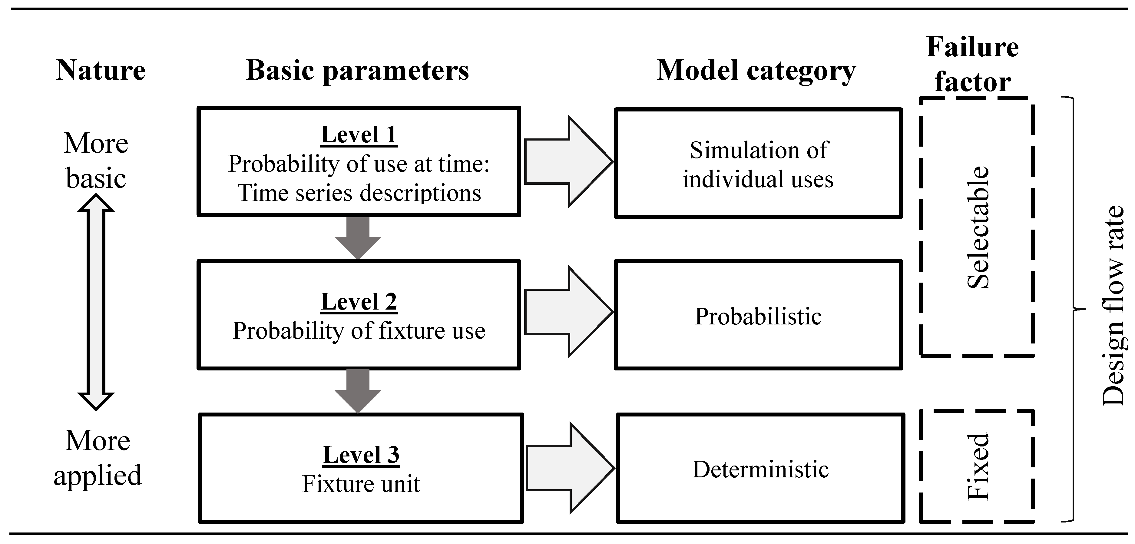
Figure 1 illustrates a schematic structure based on Carson’s definition [8] for modelling design flow rate. As the basic level models (e.g., Level 1) are associated with more descriptions of the basic demand parameters, they usually offer higher-resolution flow demands and more flexible applications. The results obtained from these models can be used to develop expressions that describe models for specific engineering design applications (e.g., Levels 1 and 2). Different levels of application result in different approaches to design flow rate estimation.

Deterministic (Level 3) models estimate the design flow rates by summing the ‘flows’ or ‘units’ of all fixtures on the system and then multiply this value by a simultaneous factor (≤1), or by using empirical formulas. As the allowable failure rates in these models are constant, the design flow rates are fixed values. These models are commonly used in design guides and standards for specific system designs.

Probabilistic (Level 2) models employ parametric probability distributions to estimate the likelihoods of different numbers of fixtures in simultaneous use. This approach uses the statistical nature of water appliances and flow rates and, together with an allowable failure rate, gives flow rate estimates corresponding to selected levels of adequacy or performance. However, as the time patterns in the flow rates are not primarily included in this approach, more probability parameters may be required to resolve the daily, weekly, diurnal, or seasonal patterns.

Simulation (Level 1) models attempt to model individual uses via Monte Carlo sampling from the cumulative frequency distributions of user demand parameters. These models can tackle time-dependent variables that are dependent on one another.

2.1. Deterministic Approach

Konen and Goncalves [7] reviewed a number of design flow determination standards and guidelines and concluded that deterministic equations and/or graphs developed for pipe sizing were mainly based on Rydberg’s model, Hunter’s model [2], or expressions (or curves) that relate the sum of unitary flow rates (or fixtures) to the design flow rate. Deterministic approaches (Figure 1) in selected codes and standards available are given below.

The analytical formula of design flow rate q_s by Rydberg [7] is the sum of three components, namely, the standard flow rate of the largest water fixture q_i,max, the mean flow rate of the other fixtures, and the risk term for the random variation of the mean flow rate of the other fixtures. It can be considered the first deterministic model based on probabilistic support. A formula of design flow rate q_s used for dimensioning of supply pipes in Scandinavian countries is given by the following equation, where pi is the probability of average water flow from each fixture q_i,μ, q_i is the nominal flow rate of fixture I, and k is the constant for a selected failure factor,

$$q_s=q_{i,\max }+p_i\left({\displaystyle \sum q_i}-q_{i,\max }\right)+k\sqrt{q_{i,\mathsf{\mu }}{p}_i\left({\displaystyle \sum q_i}-q_{i,\max }\right)}$$

(1)

A number of deterministic curves in design guides are based on Hunter’s probabilistic model or its modification [2,9]. Using Hunter’s method, the design flow rate can be determined by Equation (2), where k (=1.8226) is the constant at an allowable failure rate λ = 1% during daily rush hours, M₀ is the total number of installed fixtures, and p₀ is the probability at which each fixture is operated [10].

$$q_s=q_0{\left[M_0{p}_0+k\sqrt{2M_0{p}_0{\left(1-p_0\right)}^{}}\right]}_{}^{}$$

(2)

As fixtures of the same type are assumed in Equation (2), a fixture unit approach was adopted to approximate the design flow rate for a main pipe, which supplies appliances of different types, and to characterize the i-th appliance by the number of fixtures (p_i, q_i), i = 1, 2, 3, … M. The design flow rate, which is equivalent to the flows produced by a number of fixture units U_i, is determined by the following expressions, where q_f (=10 L·s⁻¹) is the selected reference probable maximum demand produced by each appliance type [11,12], and m is the number of fixtures that produce the reference design flow rate,

$$q_s=q_0{\displaystyle \sum _i{U}_i}{p}_0+q_{0}k\sqrt{2{\displaystyle \sum _i{U}_i}{p}_0{\left(1-p_0\right)}^{}}$$

(3)

$$U_i=\frac{m_0}{m_i};i=1,2,3,\dots$$

(4)

$$q_0\left[m_0{p}_0+k\sqrt{2m_0{p}_0{\left(1-p_0\right)}^{}}\right]=q_i\left[m_i{p}_i+k\sqrt{2m_i{p}_i{\left(1-p_i\right)}^{}}\right]=q_f$$

(5)

The design flow rate q_s is affected by the choice of q_f. Mui and Wong [11] estimated that the variations in q_s for a q_f range of 1 to 250 L·s⁻¹ could be up to 12%. According to the plumbing services design guides [13,14,15], the probability of use and the design flow rate of a unitary fixture M for a water supply system are 0.0282 and 0.15 L·s⁻¹, respectively. Design flow rates q_s for residential fixtures can be approximated by the below expression,

$$q_s=0.048M^{0.72};M\ge 30$$

(6)

Table 1. Constants for relating the sum of unitary flow rates to the design flow rate at pipes (Deutsches Institut für Normung DIN standard).

Applicable Range	k4 ≤ ∑Miqi ≤ 20 L·s−1								∑Miqi > 20 L·s−1
qi for k Value	qi < 0.5 L·s−1				qi ≥ 0.5 L·s−1				All qi
Occupancy	k1	k2	k3	k4	k1	k2	k3	k4	k1	k2	k3
Residences	−0.14	0.682	0.45	1.0	−0.70	1.7	0.210	1.0	−0.70	1.7	0.21
Offices	−0.14	0.682	0.45	1.0	−0.70	1.7	0.210	1.0	0.48	0.4	0.54
Hotels	−0.14	0.698	0.50	0.1	0	1.0	0.366	1.0	−1.83	1.08	0.50
Shopping centres	−0.12	0.698	0.50	0.1	0	1.0	0.366	1.0	−6.64	4.3	0.27
Hospitals	−0.12	0.698	0.52	0.1	0	1.0	0.366	1.0	1.25	0.25	0.65
Schools	−3.41	4.400	0.27	1.5	−3.41	4.4	0.270	1.5	11.5	−22.5	−0.50

displays the constants for relating the sum of unitary flow rates ∑M_iq_i to the design flow rate q_s as defined in a Deutsches Institut für Normung DIN (the German Institute for Standardization) standard [7].

$$q_s=k_1+k_2{\left({\displaystyle \sum M_i{q}_i}\right)}^{k_3}$$

(7)

In DIN-1998 W308 norm (German), there is an expression by Malan [16] for the design flow rate of a residential building, where U is fixture (loading) units of appliances,

$$q_s=0.25\sqrt{{\displaystyle \sum U}}$$

(8)

Mambourg [17] presented an expression in France (Règles DTU 60.11) for design flow rate calculations,

$$q_s=\frac{0.8{\displaystyle \sum M_i{q}_i}}{\sqrt{{\displaystyle \sum M_i}-1}}$$

(9)

Konen and Goncalves [7] also presented some curves (adopted in Portugal) for design flow rate calculations,

$$q_s=\{\begin{array}{c}0.5548{\left({\displaystyle \sum M_i{q}_i}\right)}^{0.4958}\\ 0.5244{\left({\displaystyle \sum M_i{q}_i}\right)}^{0.5462}\\ 0.2023{\left({\displaystyle \sum M_i{q}_i}\right)}^{0.7982}\end{array};\begin{array}{c}0<{\displaystyle \sum M_i{q}_i}\le 3\\ 3<{\displaystyle \sum M_i{q}_i}\le 44\\ 44<{\displaystyle \sum M_i{q}_i}\le 500\end{array}$$

(10)

An expression of design flow rate as stated in Brazilian Standard NBR 5606 is given below [7],

$$q_s=0.3\sqrt{{\displaystyle \sum M_i{q}_i}}$$

(11)

Konen and Goncalves [7] suggested some new values for the unitary fixtures based on the probabilistic formulation developed by Hunter [2] and proposed curves for relating 10 ≤ M ≤ 10,000 water closet (WC) flush tanks and 5 ≤ M ≤ 1000 WC flush valves to the design flow rate,

$$q_s=\frac{1}{15.85}\left(3.54\times {10}^{-10}{M}^3-1.66\times {10}^{-5}{M}^2+0.1263M+10.9\right)$$

(12)

$$q_s=\frac{1}{15.85}\left(8.5{\log }^{2}M+11.5\log M+15\right)$$

(13)

Murakawa [18] developed a loading unit method to estimate the design flow rate. Instead of using an overall average by fixture type, the time-dependent average of simultaneous use in the peak period is used for each fixture type. A design flow rate estimated this way is comparatively lower than that by the Hunter’s method (i.e., q_s,0) [2], and it is expressed by Equation (14), where k₁ and k₂ are the constants as given in

Table 2. Regression constants for approximating design flow rates.

Reference	k1	k2	Correlation Coefficient
[7]	0.5879	0.8683	0.9971
[18]	0.4819	0.0033	0.9976
[19]	1.0270	1.2266	0.9969
[20]	0.05	0.71	0.9989
[21]; Miqi ≥ 30 L·s−1	0.2283	0.5906	0.9626
[21]; Miqi < 30 L·s−1	0.11$q_{\max }^2$− 0.5qmax + 0.53	−0.36$q_{\max }^2$+ 1.66qmax − 1.23	0.9989

.

$$q_s=k_1{q}_{s,0}^{}+k_2{q}_{s,0}^2$$

(14)

In a Japanese code established by The Society of Heating, Air-conditioning and Sanitary Engineers of Japan (SHASE) SHASE-S (or HASS) 206, a set of procedures were also introduced by Murakawa [19] to determine the design flow rate using the sum of the maximum load of an appliance in a group of different sanitary appliances and the half load of the other appliances within that group. The design flow rates determined by Konen and Goncalves [7] and Murakawa [19] were compared with those by the Hunter’s probabilistic approach q_s,0 [2]. Using the curves presented in original papers and the constants listed in Table 2, approximations can be given by,

$$q_s=k_1{q}_{s,0}^{k_2}$$

(15)

In Europe, a harmonized European Union (EU) Standard [21] supersedes the previous version [20]. BS6700 [20] allocates the loading units to appliances instead of mapping the total loading units for the pipe to the simultaneous demand. The design flow rate can be approximated using Equation (16) and constants from Table 2. BSEN806-3 [21] defines that one loading unit is equivalent to a draw-off flow rate of 0.1 L·s⁻¹ and the design flow rate can be mapped to the total loading units for the water supply pipe section. With the constants given in Table 2, the design flow rates can be approximated by the below expressions, where q_max is the maximum flow rate of a single appliance unit,

$$q_s=k_1{\left({\displaystyle \sum M_i{q}_i}\right)}^{k_2};M_i{q}_i\ge 30\mathrm{L}·{\mathrm{s}}^{-1}$$

(16)

$$q_s=\exp \left[k_1{\displaystyle \sum \left(M_i{q}_i\right)}+k_2\right];M_i{q}_i<30\mathrm{L}·{\mathrm{s}}^{-1};0.2\mathrm{L}·{\mathrm{s}}^{-1}\le q_1\le 1.5\mathrm{L}·{\mathrm{s}}^{-1}$$

(17)

Wong and Mui [22] presented a deterministic curve of design flow rate for collective residential drainage appliances. The constants, displayed in

Table 3. Regression constants for the design flow rates in drainage stacks.

Reference	qs (L·s−1)	M	k0	k1	k2
[22]	0.23	70−157 158−6500	0.9 0	0.0061 0.073	1 0.64
[13,14,15]	0.34	70−157 158−6500	0.9 0	0.0061 0.073	1 0.64
[13,14,15,23]	1	All	0	0.5	0.5
[24]	0.6	100−20,000	2.3895	0.0622	0.6659

, were determined from a survey research study of 597 apartments selected among 14 high-rise residential buildings in Hong Kong. Constants from other design guides are listed in the table for comparison [13,14,15,23,24].

$$q_s=k_0+k_1{\left({\displaystyle \sum M}\right)}_{}^{k_3}$$

(18)

2.2. Probabilistic Approach

The design flow rate q_s can be determined from the probability density function of flow rates q for all connected appliances, provided that the probability does not exceed the design flow rate. P(q > q_s) is determined at an allowable maximum failure rate λ selected,

$$P\left(q>q_s\right)=\mathsf{\lambda }$$

(19)

Hunter [2] applied binomial distribution to estimate the probability P(M_s < M) of simultaneous operation of M_s appliances out of M identical appliances, which are connected to a common supply pipe. At a constant appliance flow rate q, the design flow rate q_s is determined by the discharge probability of an appliance p as expressed below, where τ₁ is the discharge period and τ₂ is the period of time between two consecutive uses,

$$q_s=q{M}_s;P\left(M\ge M_s\right)={\displaystyle \sum _{M_s}^M{C}_{M_s}^M}{p}_{}^{M_s}{\left(1-p_{}^{}\right)}_{}^{M-M_s};p=\frac{{\mathsf{\tau }}_1}{{\mathsf{\tau }}_2}$$

(20)

The time period between two consecutive uses τ₂ can be related to the user queue as expressed by the following equation [25], where n_a is the number of appliances serving a group of users at an arrival rate γ,

$${\mathsf{\tau }}_2=\frac{n_a}{\mathsf{\gamma }}$$

(21)

In order to address the design flow rates for different types of appliances, Webster [26] applied a generalized binomial distribution to determine the simultaneous operation of M_j,s appliances out of M_j appliances in a group of identical appliances j (i.e., out of j independent groups). The probability of M_j,s is given by Equation (22), where p_j is the probability of an appliance j operating in the peak period.

$$P\left(M_{j,s}^{}\right)={\displaystyle \prod _{j=1}^J\left[C_{M_{j,s}^{}}^{M_j}{p}_j^{M_{j,s}^{}}{\left(1-p_j^{}\right)}_{}^{M_j-M_{j,s}^{}}\right]};p_j=\frac{{\mathsf{\tau }}_{1,j}}{{\mathsf{\tau }}_{2,j}}$$

(22)

The flow rates q through the common supply pipe when M_j,s appliances are operating simultaneously can be calculated using Equation (23), and the design flow rate q_s is determined from P(q > q_s) in Equation (19).

$$q_s={\displaystyle \sum _j^{}{q}_j{M}_{j,s}}$$

(23)

This approach is further developed for a pipe with different flow rates q_j from N_j associated probabilities p_j during the peak period [27,28], where p₀ is the probability of zero flow rate for appliances M_s,0,

$$P\left(M_{j,s}\right)=\frac{p_0^{M_{s,0}^{}}{p}_j^{M_{s,j}^{}}}{M_{s,0}^{}!M_{s,j}^{}!}$$

(24)

Murakawa [19] followed Hunter’s approach [2] and suggested a Poisson distribution (instead of a binomial distribution),

$$P\left(M\ge M_s\right)={\displaystyle \sum _{M_s}^M\frac{e^{-Mp}\left(Mp\right){}^{M_s}}{M_s!}}$$

(25)

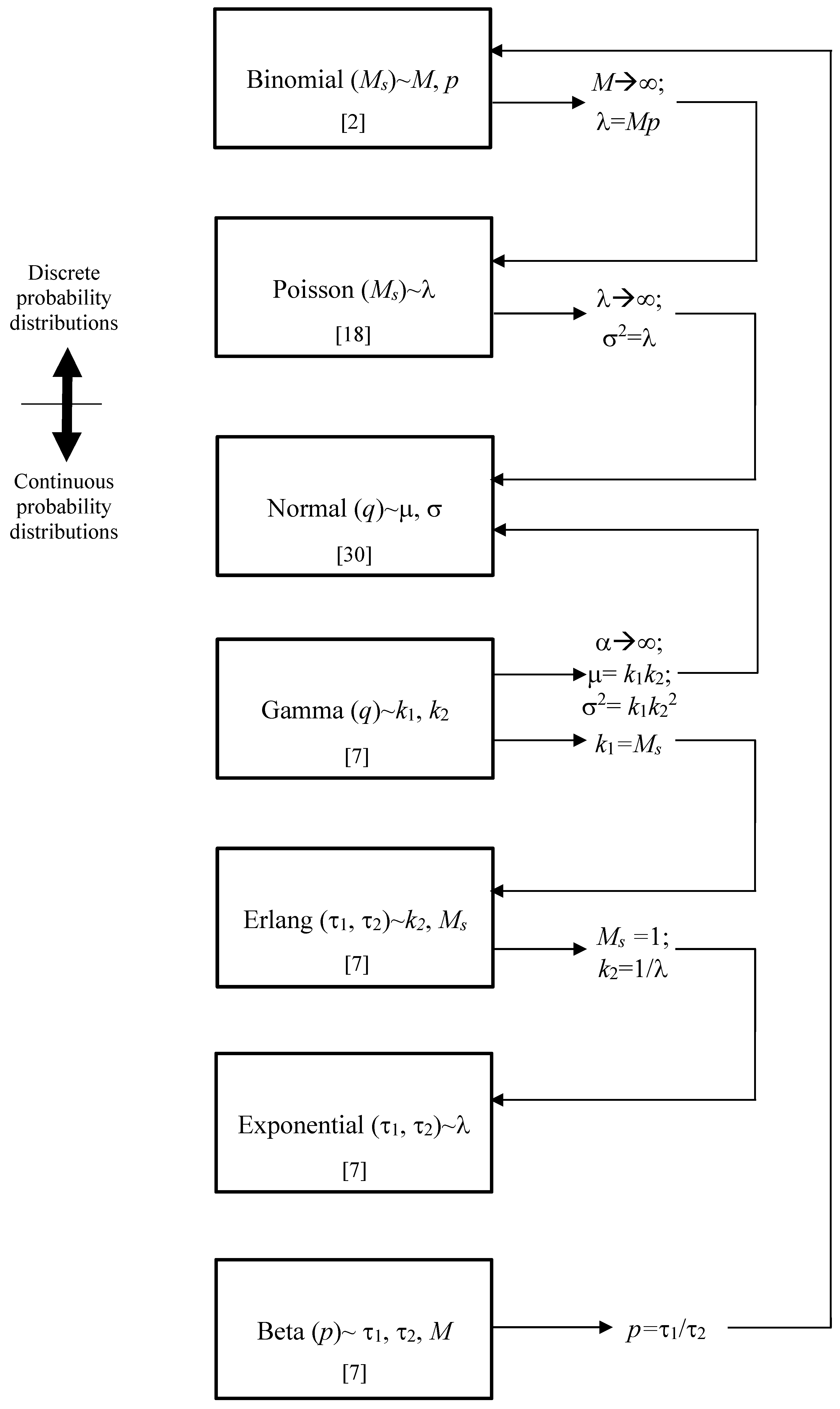
Ilha et al. [29] developed an open model for τ₁, τ₂, and q for appliances M. All of the four parameters are described by parametric distributions. The simultaneously operating appliances M_s are described by a beta-binomial distribution B as shown in Equations (26)–(30) below, where τ₁ and τ₂ can be represented by Erlang or exponential distributions; the probability p is beta distributed; q and q_s are given by gamma distributions; and k₁, k₂, and M_s are the distribution parameters,

$$P\left(p\right)=\frac{\Gamma \left({\mathsf{\tau }}_2+{\mathsf{\tau }}_1\right)}{\Gamma \left({\mathsf{\tau }}_1\right)\Gamma \left({\mathsf{\tau }}_2\right)}{p}_{}^{{\mathsf{\tau }}_1-1}{\left(1-p\right)}_{}^{{\mathsf{\tau }}_2-1}$$

(26)

$$P\left(M_s\right)=C_{M_s}^M\frac{B\left(M_s+{\mathsf{\tau }}_1,M-M_s+{\mathsf{\tau }}_2\right)}{B\left({\mathsf{\tau }}_1,{\mathsf{\tau }}_2\right)}$$

(27)

$$q_s={\displaystyle \sum _j^{}{q}_j{M}_{j,s}}$$

(28)

$$P\left(x={\mathsf{\tau }}_1,{\mathsf{\tau }}_2\right)=\{\begin{array}{c}\frac{x^{M_s-1}{e}^{-x/k_2}}{k_2^{M_s}\left(M_s-1\right)!}\\ \mathsf{\lambda }{e}^{-\mathsf{\lambda }x}\end{array}$$

(29)

$$P\left(q>q_s\right)={\displaystyle \underset{q_s}{\overset{\infty }{\int }}\frac{q_{}^{k_1-1}{e}^{-q/k_2}}{k_2^{k_1}\Gamma \left(k_1\right)}dq}$$

(30)

Alitchkov [30,31] proposed that the design flow rate can be determined by the cumulative normal distribution of simultaneous flow rates q_s at time t over a period of one year, where M is total number of fixtures and σ² is the variance of flow rate which serves as a stochastic component,

$$P\left(q>q_s\right)=\frac{1}{\mathsf{\sigma }\sqrt{2\mathsf{\pi }}}{\displaystyle \underset{q_s}{\overset{\infty }{\int }}\exp \left(-\frac{{\left(q\left(t\right)-q_{s,\mathsf{\mu }}\right)}_{}^2}{2{\mathsf{\sigma }}^2}\right)dq};q\sim q(\mathsf{\mu },{\mathsf{\sigma }}^2)$$

(31)

2.3. Deterministic Model Simplification

Relationships of various distributions are illustrated in Figure 2. Design flow rates suggested at an acceptable failure rate ε can be given by the following expression, with a constant k accounting for various distributions adopted [10,29],

$$q_s=\mathsf{\mu }+k\mathsf{\sigma };q\sim q(\mathsf{\mu },{\mathsf{\sigma }}^2)$$

(32)

This approach was adopted in some design guidelines as a form of deterministic equation. One possibility is to use the normal approximation for the binomial distribution to estimate peak loads directly [10]. Below is an expression by Wistort [32] for the direct estimation of the 99th percentile of the flow rates from j appliance types,

$$q_s=\mathsf{\mu }+k\mathsf{\sigma };\mathsf{\mu }={\displaystyle \sum _j^{}{q}_j{M}_j{p}_j};\mathsf{\sigma }=\sqrt{{\displaystyle \sum _j{q}_j^2{M}_j\left(p_j^{}-p_j^2\right)}}$$

(33)

By taking p₀ (=0 for M_p > 5) as the expected number of operating fixtures in a collection of j fixture groups, it can be rewritten in a dimensionless variation [32,33],

$$q_s=\left(1+\frac{k\mathsf{\sigma }}{\mathsf{\mu }}\right)\frac{{\displaystyle \sum _j{M}_j{p}_j}}{1-p_0}$$

(34)

$$p_0={\displaystyle \prod _j{\left(1-p_j\right)}^{M_j}}$$

(35)

Theoretically, the design flow rate tends towards the discharge probability p when the number of appliances is increasing. Taking Hunter’s equation [2] for illustration, Equation (2) can be expressed by the fractional design flow rate $q_s^{*}$, that is, the design flow rate can be divided by the maximum flow rate,

$$q_s^{*}=\frac{q_0\left[M_0{p}_0+k_{\mathsf{\lambda }}\sqrt{2M_0{p}_0{\left(1-p_0\right)}^{}}\right]}{q_0{M}_0}=p_0+\frac{k}{M_0}\sqrt{2M_0{p}_0{\left(1-p_0\right)}^{}}$$

(36)

$$\underset{M_0\to \infty }{\lim }{q}_s^{*}=\underset{M_0\to \infty }{\lim }\left(p_0+\frac{k_{\mathsf{\lambda }}}{M_0}\sqrt{2M_0{p}_0{\left(1-p_0\right)}^{}}\right)=p_0$$

(37)

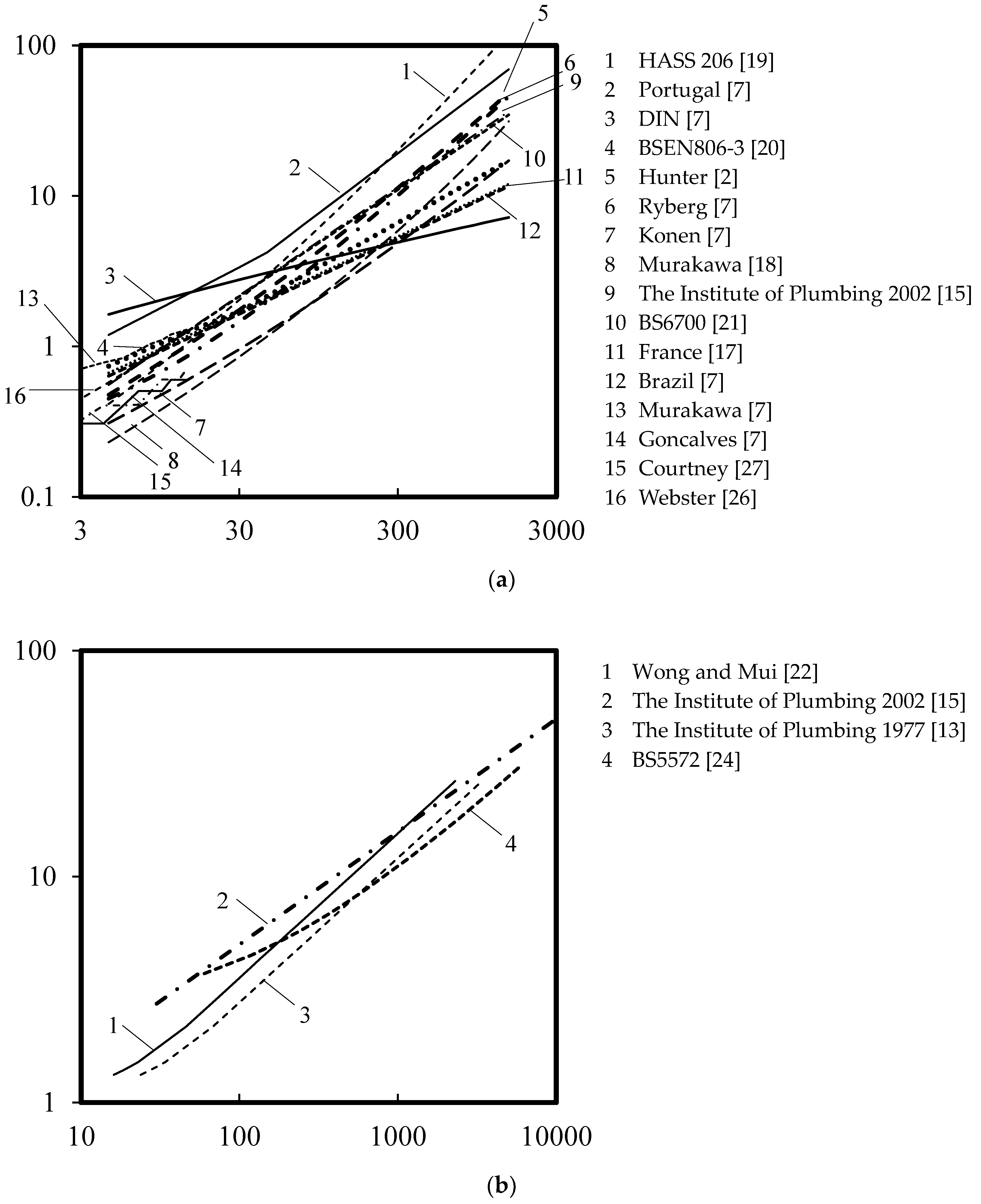
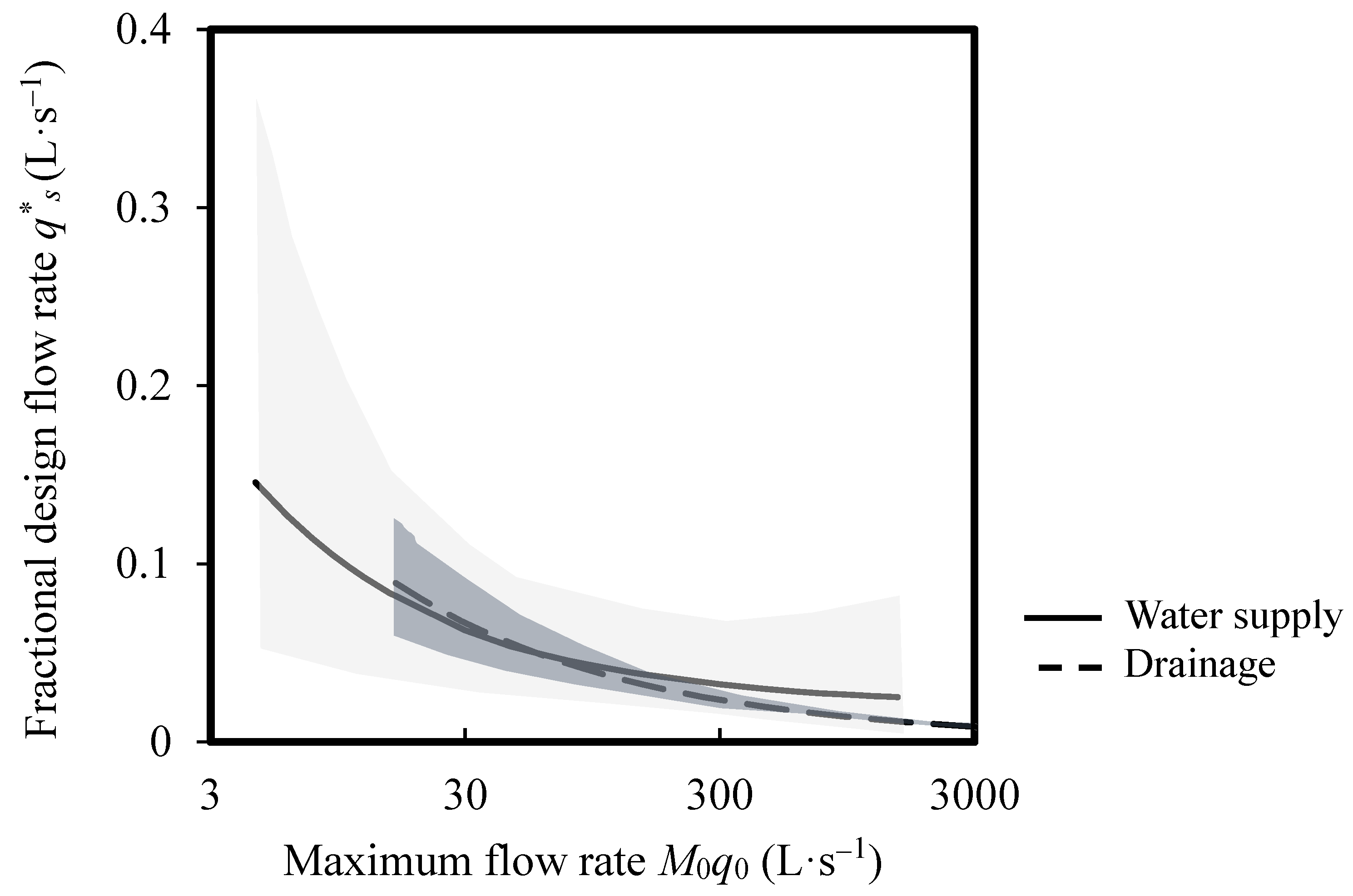
The fixture flow rates determined from various deterministic and probabilistic models cannot be compared directly as different models assume different flow rates and demand probabilities for the reference fixtures installed. Figure 3 plots the design flow rates q_s as a function of the sum of fixture flow rates M₀q₀ based on various deterministic and probabilistic models for residential water supply and drainage systems. Although large variations of the predicted design flow rates (i.e., 1–10 times) can be seen in the figure, all model estimates show consistent trends. The fractional design flow rates q_s^* from various deterministic models are normally distributed (p > 0.05, w/s test). Figure 4 illustrates the average fractional design flow rate estimates against the maximum flow rates, within an estimate range of 0.005–0.36 L·s⁻¹. The results show a decreasing trend of fractional design flow rates from 0.15 to 0.025 L·s⁻¹ against an increasing sum of the sum of fixture flow rates from 4.5 to 1500 L·s⁻¹.

2.4. Simulation and Time Series Approach

Design flow rates can be determined from instantaneous demand time series via Monte Carlo sampling techniques [27]. In the Monte Carlo simulations, a large number of pseudo-random uniform numbers u_i are obtained from the intervals (0, 1) to map numeric values x_s,i to model parameters x_s as described by the following probability mass or density function,

$$x_{s,i}^{}={\displaystyle \underset{-\infty }{\overset{u_i}{\int }}{\tilde{x}}_s}d{x}_s$$

(38)

Studies show that for appliances i (with different usage patterns) installed in the same washroom, the probable maximum simultaneous water demands can be determined using the Monte Carlo sampling techniques even when the appliances are not operating simultaneously [34,35]. The design flow rate q_s for all washrooms j with demands q and an allowable failure factor λ (=1%) is expressed by the following equation, where q_i is the water demand in rush hour τ, τ₀ is the time period without demand, and τ₁ is the time period with demand,

$$P\left(q>q_s\right)=\mathsf{\lambda };q={\displaystyle \sum _{ij}{q}_{ij}\left(t\right)};t\in \mathsf{\tau }={\mathsf{\tau }}_0+{\displaystyle \sum _i{\mathsf{\tau }}_{1,i}}$$

(39)

With known demand probability and demand flow rate in each hour, daily demand time series can also be made up using Monte Carlo simulations [36]. Mui and Wong [37] proposed a time series model constructed this way to determine the occurrence and duration of drainage demands from random and intermittent appliance discharges.

Simulation procedures for the demand time series can be programmed for the ease of use [38]. Once the time series are obtained, descriptive statistic quantities of instantaneous demands (e.g., maximum and average values with various failure factors) in any integrating periods can be computed. A number of research works have been done for this purpose. Rathnayaka et al. [39] reviewed some tools for generating end-use data for residential water systems. Duncan and Mitchell [40] developed a model that simulates household water demands for a range of end uses and aggregates multi-year demand sequences generated at 1-min time steps to a time series. Thyer et al. [41] presented a probabilistic behavioural model to simulate household water use at 1-min time steps. SIMDEUM, developed by Blokker et al. [42,43], is a water demand end-use model that combines various water use behavioural patterns with the knowledge of appliance types to predict water use on a micro scale (at 1-s time steps). In order to optimize the inflow rate of a tank water supply system, Wong et al. [44] integrated a demand time series.

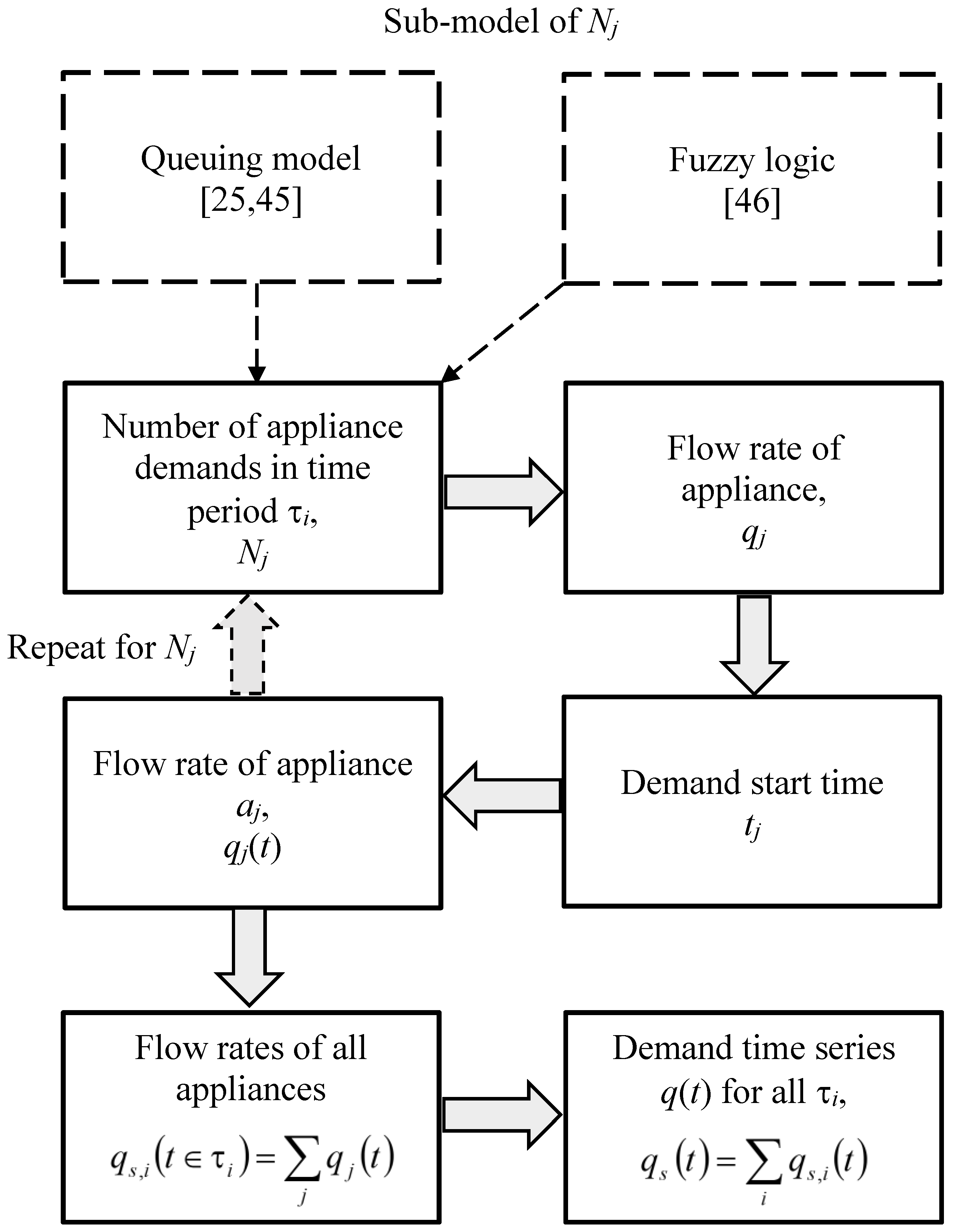
Figure 5 shows the core calculation procedures for constructing the time series of simultaneous demands. Sub-models of key parameters (e.g., number of appliance demands within a time period, flow rate, demand duration, etc.) can be included either through various approximations of parametric distribution functions, surveyed frequency distributions, or further physical relationships. The queuing models by Goncalves and Alves da Graca [25] and Mui and Wong [45] for sanitary appliances in congested use and a fuzzy algorithm by Oliverira et al. [46] for demand start time and duration calculations are a few good examples.

For simulations of the simultaneous demands, a time-series is subdivided into a number of time partitions τ_i, i = 1, 2, 3, …, with a number of demands N of appliances j = 1, 2, 3, …; and each demand has a time variant demand q_j(t) for each operation and a uniformly distributed demand start time t_j in τ_i [36]. Using Monte Carlo sampling for the fractional demand start time u from a uniform distribution function, the demand start time in the time partition is given by,

$$t_j=u{\mathsf{\tau }}_i^{}$$

(40)

The flow rates from all appliances in the time partition and for all time partitions are given by,

$$q_s^{}\left(t\right)={\displaystyle \sum _i^{}{q}_{s,i}^{}\left(t\right)}$$

(41)

$$q_{s,i}^{}\left(t\right)={\displaystyle \sum _j^{}{q}_j^{}\left(t\right)}$$

(42)

Asano et al. [47] studied time series of instantaneous demands in an office building and compared the maximum flow rate predictions made by a linear multivariate equation with those made by a neural network. Although the neural network approach could give a better prediction, no physical explanation was given in that study. In latter studies by Murakawa et al. [48,49], time series of instantaneous maximum flow rates modelled by Monte Carlo simulation techniques were used to estimate the design flow rates for office buildings and restaurants.

3. Bayesian Approach

Most water supply system designs are routinely and substantially over-sized as the prospect of system failure is commercially and professionally unimaginable [4,50]. It was opportunistic to determine the probable maximum simultaneous demands in measurements. Usage patterns of water appliances associated with occupancy, replacement of newer appliances, and lifestyle changes in installations added uncertainty to data quality of the maximum demands in long-term measurement. Indeed, there were insufficient long-term measurements available in open literature to establish promising design flow rates for all water installations in buildings. Regarding the most appropriate choice of design flow rate for sustainable development in buildings, there is no conclusive evidence that favors either model or measurement outcome.

3.1. Measurement Data

Vrana et al. [51] studied the peak flow rates measured in 12 (n = 12; number of residents = 12–168) water supply systems for residential buildings in the Czech Republic and compared them with the design flow rates given in four design guidelines, namely, CSN75-5455 (Czech), EN806-3 (British), W3 (Swiss), and DIN1988-300 (German). Reportedly, the measured rates were fractions of the design flow rates: 0.173–0.483 for CSN, 0.2–0.568 for EN, 0.262–0.684 for W3, and 0.256–0.692 for DIN. The fraction values appeared to be normally distributed (p ≥ 0.1, Shapiro-Wilk test); except for CSN (p = 0.04, t-test for correlation), where no significant correlation between predicted and measured values was found (p > 0.05, t-test for correlation).

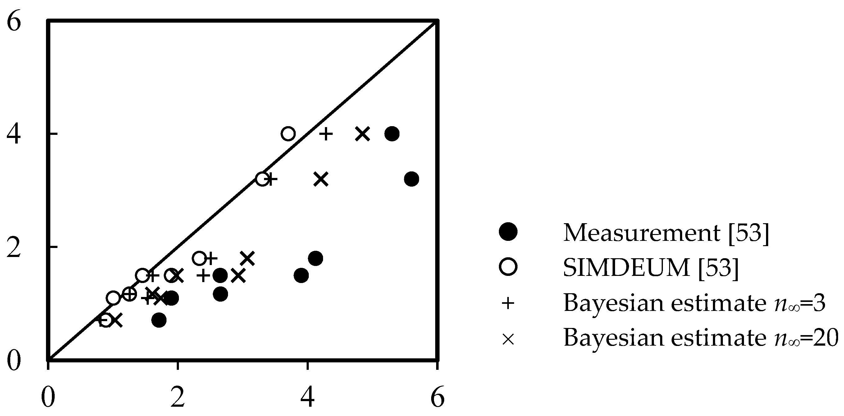
Pieterse-Quirijns et al. [52] and Blokker et al. [53] investigated the flow rates measured on a per second basis for the hot and cold water supply systems in two offices (255–2000 employees), two business hotels (80–192 rooms), and two nursing homes (124–260 beds). The measurement periods ranged from 28 to 47 days, and the measurement results showed that the peak flow rates were only fractions (0.417–0.755) of the design flow rates given in existing guidelines.

In a research project by Malan [16], daily peak domestic water demands were gauged in a 134-unit apartment building for 12 consecutive calendar days. The measured peak demand was 8.77 L·s⁻¹ and that was equal to 46.6% of the estimated value given in the German design guide W308. That project included 166 WC cistern inlet valves, 536 taps (15-mm), and 268 taps (20-mm).

Murakawa et al. [48] reported that, from a continuous measurement period of 14 months, the instantaneous maximum flow rate of a water supply system, which served 21 restaurants (with a total of 1932 seats), was 8.8 L·s⁻¹. The design flow rate of the system was 10.4 L·s⁻¹ [13,14,15,54]. According to the studies by Takata et al. [55] and Murakawa et al. [48], the instantaneous maximum flow rate recorded for the water supply system in a 14-story office building (total floor area = 18,256 m²) was 3.2 L·s⁻¹, while the system design flow rate was 11.8 L·s⁻¹ [13,14,15].

In yet another study, Murakawa et al. [56] investigated the water flow rates for 16 residential buildings (95–910 flats). The maximum simultaneous flow rates, recorded from measurements made at 1.2-min intervals for one year, were presented as a function of loading units. A total of 29 measurement data sets (n = 29) were given as a fraction (α = 0.276–0.522) of a design flow rate range of 2.9 to 65 L·s⁻¹ [18,56]. The fraction values were assumed to be normally distributed (p ≥ 0.1, Shapiro–Wilk test), and there was no significant correlation between the fractions α and the loading units (p = 0.75, t-test for correlation).

Recently, a Bayesian approach has been proposed to bridge the gap between model estimates and field measurements for the probable maximum simultaneous water demand [57]. Bayes’ theorem, which relates the conditional and marginal probabilities of stochastic events A and B (where B has a non-vanishing probability), asserts that the probability of an event A given by event B depends not only on the relation between events A and B, but also on the marginal probability of occurrence of each event. This theory can be applied to a sample size not large enough for decision-making purposes, yet relevant enough for statistical analysis. Its general formulation and various applications are available in the literature [54,58]. Studies applied Bayesian analysis to improve understanding of the downtime characteristics of water installations [59]. Factor weights contributed to water pipe conditions were evaluated with Bayesian inference [60]. A Bayesian network was used as an aid to integrated water resource planning, accounting various considerations of environmental, economic, social, and political impacts, as well as inputs from stakeholders in decision making process [61]. In this section, the proposed approach predicts the probable maximum simultaneous demand for the total fixtures installed using the readily available model predictions (event A) and the measurements from a compatible installation (event B).

Given a measured (maximum) value $q_m^{*}$~N(μ,σ²), the posterior estimate of a fractional design flow rate $q_{s,1}^{*}$~N(${\mathsf{\mu }}_1^{}$,${\mathsf{\sigma }}_1^2$) is expressed by the following Bayesian rules [62], where $q_{s,0}^{*}$~N(${\mathsf{\mu }}_0^{}$,${\mathsf{\sigma }}_0^2$) is the prior estimate of the fractional design flow rate; p is the probability; μ and σ² are the mean and variance of a normal distribution function, respectively; μ and μ₀ are the best estimates of the fractional measured value and design value $q_m^{*}$ and $q_{s,0}^{*}$, respectively,

$$p\left(q_{s,1}^{*}|q_m^{*}\right)=p\left(q_{s,0}^{*}\right)p\left(q_m^{*}|q_{s,0}^{*}\right)$$

(43)

$${\mathsf{\sigma }}_1^2={\left({\mathsf{\sigma }}_0^{-2}+{\mathsf{\sigma }}_{}^{-2}\right)}_{}^{-1};{\mathsf{\mu }}_1={\mathsf{\mu }}_0{{\mathsf{\sigma }}_0}^{-2}/({\mathsf{\sigma }}_0^{-2}+{\mathsf{\sigma }}^{-2})+\mathsf{\mu }{\mathsf{\sigma }}^{-2}/({\mathsf{\sigma }}_0^{-2}+{\mathsf{\sigma }}^{-2})$$

(44)

In these rules, the weightings are proportional to their respective variances, and the posterior mean is a weighted average of the prior mean and the measured value given. This posterior mean can be characterized by the ratio of standard deviations and expressed as a parameter β.

β² = σ²/σ₀²

(45)

Given a measurement maximum flow rate μ is significantly different from a prior belief of the maximum (design) flow rate μ₀ that |μ₀ − μ| > ε, where ε is a cut-off value of the acceptable error.

Suppose repeatedly measurements given the same value μ that an acceptable choice of design flow rate q_s^*–μ_n. Denote X = σ₀⁻²/(σ₀⁻² + σ⁻²) = β²/(1 + β²) and Y = μ σ⁻²/(σ₀⁻² + σ⁻²) = μ/(1 + β²), posterior estimates μ₁, μ₂, …, μ_n are given below,

μ₁ = μ₀ X + Y, μ₂ = μ₀ X ² + XY + Y, …, μ_n = μ₀ Xⁿ + Y (Xⁿ⁻¹ + Xⁿ⁻² + … + X + 1)

(46)

μ_n = μ₀ Xⁿ + Y (1 − Xⁿ)/(1 − X)

(47)

It is noted for Equation (47) μ_n→μ when n→∞. Taking n is a finite number of the repeated observations such that the n-th estimate shows no significant difference from measured acceptance, that is, |μ_n − μ| ≤ ε, and β² can be determined below,

μ₀ Xⁿ + Y (1 − Xⁿ)/(1 − X) = μ + ε

(48)

$${\mathsf{\mu }}_0{\left(\frac{{\mathsf{\beta }}^2}{1+{\mathsf{\beta }}^2}\right)}^n+\left(\frac{\mathsf{\mu }}{1+{\mathsf{\beta }}^2}\right)\left(\frac{1-{\left(\frac{{\mathsf{\beta }}^2}{1+{\mathsf{\beta }}^2}\right)}^n}{1-\left(\frac{{\mathsf{\beta }}^2}{1+{\mathsf{\beta }}^2}\right)}\right)=\mathsf{\mu }+\mathsf{\epsilon }$$

(49)

β² = c_r^1/n/(1 − c_r^1/n); c_r = ε (μ₀ − μ)⁻¹

(50)

The constant c_r is the ratio of acceptable error to the difference between the prior value μ₀ and the measured value μ. Therefore, the weighting parameter β can be expressed by the target sample size, the acceptable error of the estimate, the measured value, and the prior estimate.

For the simplicity of application of the Bayesian calculated results with the prior estimated values, a ratio of measured value to the prior estimate is defined below,

$$\mathsf{\alpha }=q_m^{*}/q_{s,0}^{*}$$

(51)

The target sample size n_∞, for repeated measures of the maximum flow rate, is a finite value that is deemed sufficient to adopt the measured maximum flow rate for design calculations with acceptable error in the final estimate ε_∞.

$${\mathsf{\epsilon }}_{\infty }^{}=\left|q_{s,\infty }^{*}/q_{m,\infty }^{*}-1\right|$$

(52)

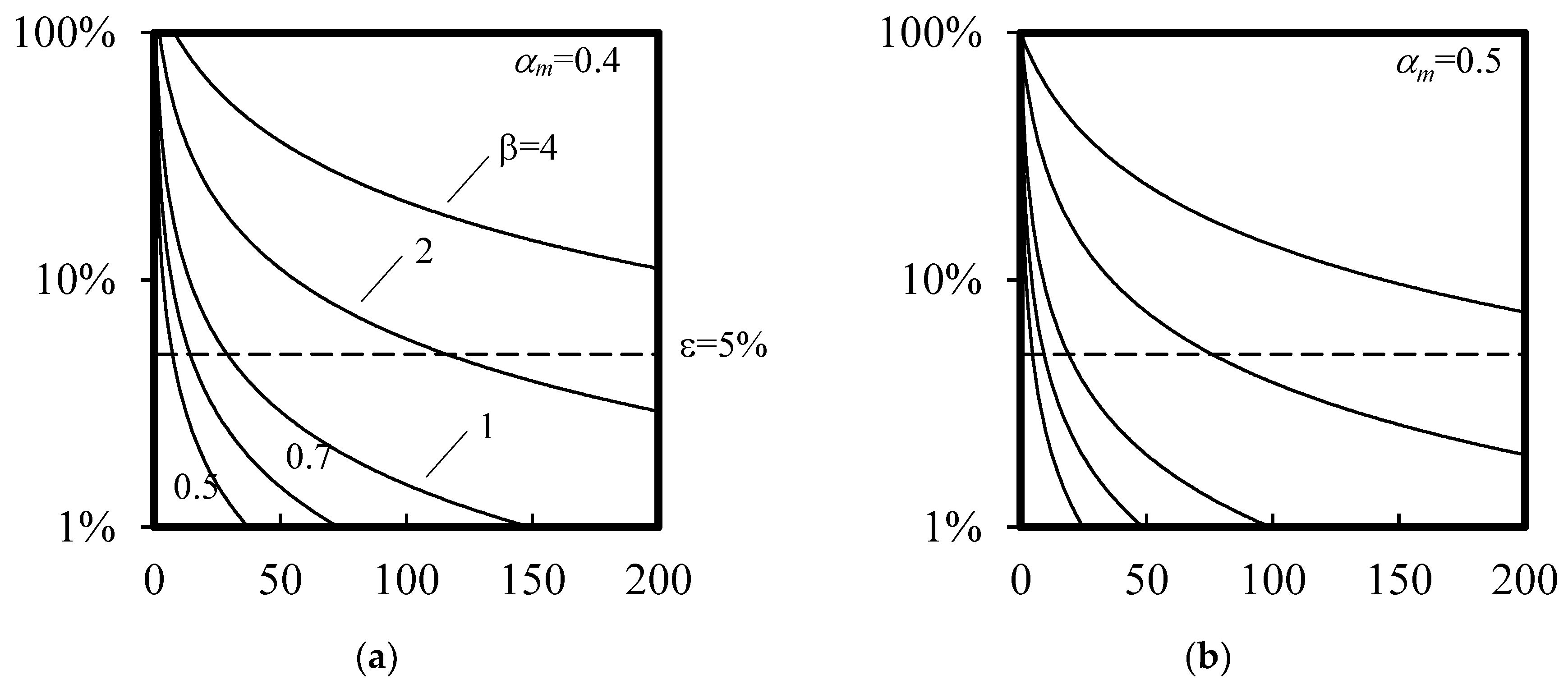
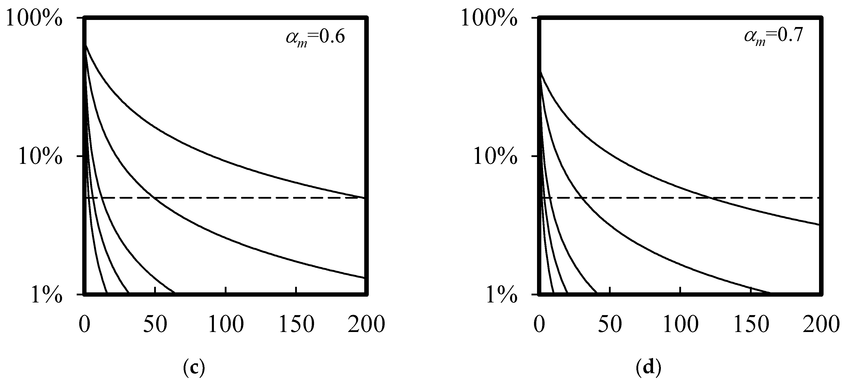
Figure 6 illustrates the examples of β (ranged between 0.5 and 4) for a sample size n with errors ε and α (ranged between 0.4 and 0.7). With the predetermined values for β~β(n_∞, ε_∞, α), the posterior estimate of the fractional design flow rate for measured $q_m^{*}$ and a sample size n is given by,

$$q_{s,i}^{*}=(q_{s,i-1}^{*}+q_m^{*}{\mathsf{\beta }}_{}^{-2}){(1+{\mathsf{\beta }}^{-2})}^{-1};i=1,2,3,\dots n$$

(53)

3.2. Bayesian Coefficient

The posterior design flow rate estimates for a sample size q_s,n can be determined by multiplying the corresponding prior design flow rate estimates q_s,0 and a Bayesian coefficient α_n,

$$q_{s,n}^{}={\mathsf{\alpha }}_n^{}{q}_{s,0}^{}$$

(54)

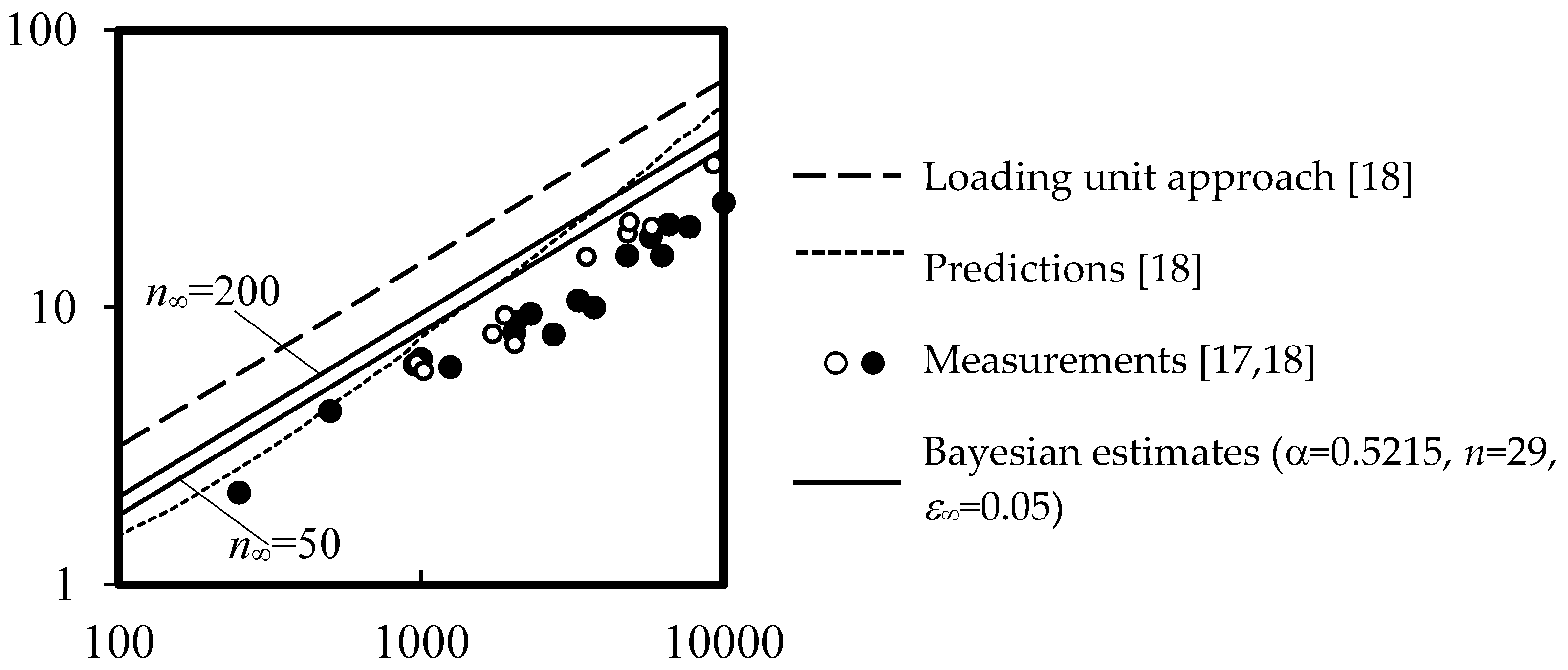
Figure 7 exhibits the Bayesian design flow rates estimated for some residential buildings with target sample sizes n_∞ = 50 and 200, α = 0.5215, n = 29, and ε_∞ = 0.05. Estimates made by Murakawa [16] are shown for comparison. For the cases with a sample size close to the target sample size, the posterior estimates are very close to the ones made by Murakawa and approaching the measured maximum loading units. For a larger target sample size, the posterior estimates are closer to the prior values than the measured ones.

Table 4. Bayesian coefficients of design flow rates α_n.

Building Type and Location	Sample Size n	Prior Estimated Design Flow Rateqs,0 (L·s−1)	Measured (Maximum) Fraction αm	αn(Reference Design Guide)
				n∞ = 50	n∞ = 100	n∞ = 200
Czech Republic				CSN75-5455 (Czech)
Residential	11	1.09–3.79	0.483	0.571	0.633	0.715
British				EN806-3 (British)
Residential	11	0.95–3.80	0.568	0.666	0.728	0.801
Swiss				W3 (Swiss)
Residential	11	0.80–2.34	0.684	0.796	0.843	0.895
German				DIN1988-300 (German)
Residential	11	0.88–2.24	0.692	0.799	0.850	0.901
Netherlands				Dutch guidelines
Office	2	1.1–4.0	0.579–0.755	0.956	0.976	0.994
Hotel (cold)	2	1.5–1.8	0.437–0.567	0.844	0.904	0.946
Hotel (hot)	2	0.71–1.17	0.416–0.441	0.725	0.817	0.891
Nursing home	2	1.5–3.2	0.385–0.571	0.800	0.874	0.927
South Africa				W308 (German)
Residential	1	18.8	0.466	0.837	0.904	0.947
Japan				Loading unit (Japanese)
Residential	29	2.9–65	0.522	0.565	0.602	0.695
Office	1	11.8	0.271	0.627	0.750	0.847
Restaurant	1	10.4	0.846	0.992	0.996	0.998

summarizes the coefficients α_n for the office and restaurant cases. Correction to the estimated design flow rate is unnecessary for any case in which the difference between prior and measured values is insignificant, the coefficient α_n is close to unity or the sample size is small (e.g., the restaurant case).

Figure 8 plots the measured maximum flow rates against the estimates made by SIMDEUM [36]. As can be seen, good predictions were made by SIMDEUM with only a few underpredictions. Figure 8 also graphs the Bayesian estimates for n_∞ = 3 and 20, where the Bayesian correction factors applied. When n_∞ = 3, the Bayesian estimates are very close to the predictions made by SIMDEUM; when n_∞ = 20, a target sample size of 10% can be achieved that the corrected Bayesian estimates are closer to the original design estimates.

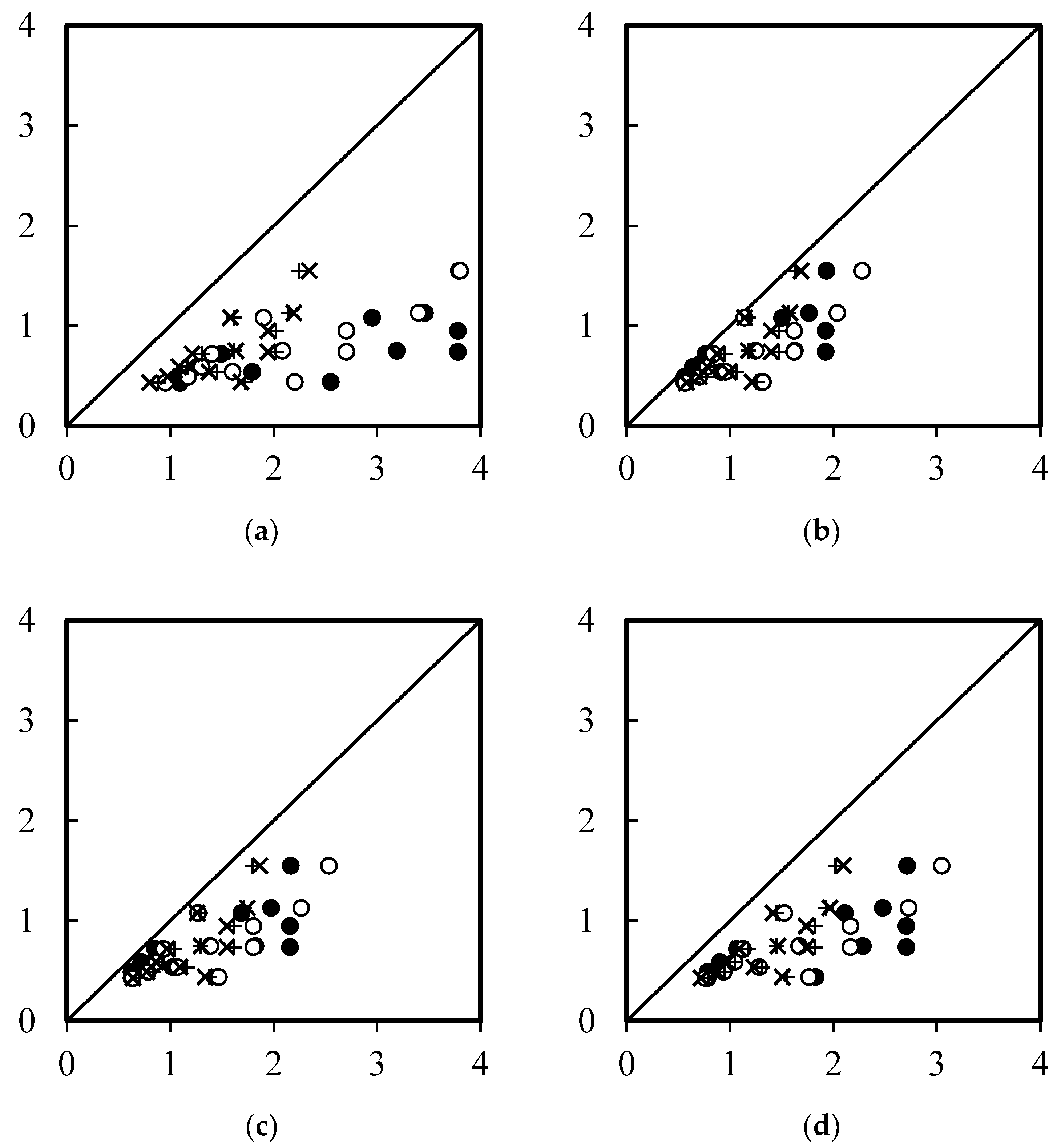
Figure 9 shows the measured maximum flow rates against the estimates made by the design guidelines CSN75-5455, EN806-3, W3, and DIN1988-300. It also graphs the Bayesian estimates for n_∞ = 13 (i.e., a sample size very close to the target sample size), 50, and 200. The figure demonstrates that Bayesian coefficients can significantly improve prediction quality (Figure 9b).

The Bayesian coefficients of design flow rates for various buildings and design guidelines are summarized in Table 4. As the proposed Bayesian approach, without any conceptual assumptions of failure factors as required in many probabilistic models (e.g., Hunter’s model), gives results comparable to those obtained through design guidelines as well as small-scale measurements, existing systems can be retained with only minor modifications to the updated measurement results.

4. Demand Sizing, Energy Loss Minimization, and Cost Implications

A pipe size that is based on demand estimates has cost implications. Construction, maintenance, and remedy (repairing) costs of water supply systems for some high-rise buildings in Hong Kong are correlated with the ratio of pipe surface area to pipe length [63]. The costs η for pipe construction, maintenance, and remedy are given by the following expression, where D is the average pipe diameter, with constants k₀ and k₁ as exhibited in

Table 5. Constants k₀ and k₁ for water systems in buildings.

System	Cost	Commercial Buildings		Residential Buildings
		k0	k1	k0	k1
Water supply	Construction	1	0.33	1	0.91
	Maintenance	1	0.38	1	3.62
	Remedy	1	1.29	1	6.50
Drainage	Construction	0.67	0.18	0.62	1.69
	Maintenance	1	5.83	1	1.74
	Remedy	1	1.29	1	6.50

,

$$\mathsf{\eta }\sim k_0{D}_{}^{2k_1}$$

(55)

For a high-rise tank water system that supplies water to 600 residential WC cisterns as described by Wong et al. [44], downsizing the supply pipe from a diameter of 67 mm to 54 mm can reduce the pipe construction, maintenance, and remedy costs by 32%, 79%, and 94%, respectively.

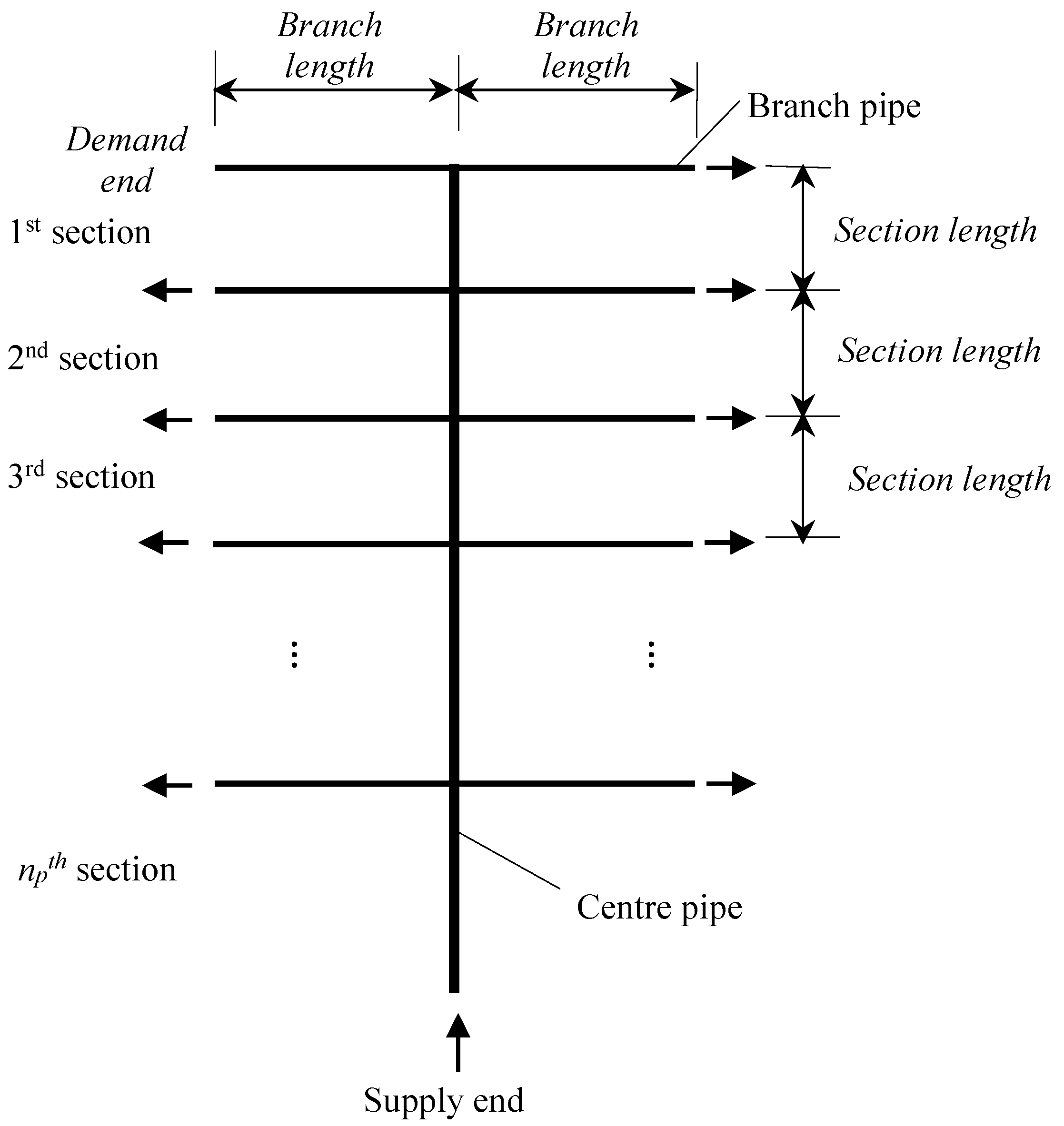
As energy is consumed to compensate the pressure loss due to pipe friction, pipe sizes should be chosen to minimize energy losses in a piping network. According to an energy loss optimization method by Mui et al. [64], for the probabilistic demands (from p = 0 to 1) at the branch pipes (of identical radius) in a basic T-shaped piping network of constant volume, the optimal radius ratio of the centre pipe is in the range from 2^1/7 to 2^3/7. This method can be extended to a tree-shaped piping network where a centre pipe is used to feed a number of paired branch pipes (i.e., a number of T-shaped piping networks as arranged in Figure 10), and the optimal radius ratio ϕ_p is given by [65],

$${\mathsf{\varphi }}_p=\{\begin{array}{c}{\left(1+n_p^{}\right)}_{}^{1/7}\\ {\left(2{\displaystyle \sum _{i=1}^{n_p}{\left(2i\right)}^2}\right)}^{1/7}\end{array};p:\{\begin{array}{c}<1\\ =1\end{array}$$

(56)

To demonstrate the implications of the volume constraint, an example using eight pairs of WC cisterns was presented by the authors of [65]. Two cases, case 1 with medium demands and case 2 with high demands, were illustrated. The demand flow rate was 0.1 L·s⁻¹ with a branch pipe diameter of 16 mm (determined by the Hunter’s method [2]) and a flow velocity of 1 ms⁻¹. While the pipe radius ratios were 16 mm/8 mm = 2 and 20 mm/8 mm = 2.5, the demand probabilities were 0.1 and 0.2 (corresponding to public water closets in offices and shopping malls [13,14,15]) for cases 1 and 2, respectively. Suppose choices of pipe radius were available, the existing designs would consume 12% (case 1) or 43% (case 2) more pipe fiction energy than the optimal cases. In other words, with appropriate demand-controlled pump operations, this pipe sizing approach can offer pumping energy savings potentials for the two cases. For the optimal pipe radius ratios of 1.70 and 1.86 for demand probabilities 0.1 and 0.2, with the constraint of an equal pipeline volume, the corresponding centre/branch pipe radii are 15.5 mm/9.1 mm and 19 mm/10.2 mm, respectively.

In commercial building settings, the cost implications for sizing pipes with minimum energy loss were estimated according to the lengths of centre and branch pipes in a ratio of 1:1 using Equation (55). The results, shown in

Table 6. Implications of sizing a tree-shaped piping network (with branch demand flow rates of 0.1 L·s⁻¹) with energy loss minimization [61,62].

Case	Demand Probability	Average Pipe Diameter	Energy Loss	Costs
				Construction	Maintenance	Remedy
(1)	0.1	+2.5%	−11%	+0.8%	+0.9%	+3.0%
(2)	0.2	+4.3%	−30%	+1.4%	+1.6%	+5.6%

, indicate that the proposed sizing method will reduce energy losses, but with additional costs generated by larger pipe sizes in compared with those sizes given in some practices [13,14,15]).

5. Discussion

Overestimation of the probable maximum water demands being made simultaneously at the different water outlets in a network leads to inefficient use of water and energy resources. Without accurate demand estimates, it is impossible to optimize water systems in the quest for a sustainable built environment.

In the above sections, by reviewing all major demand models and corresponding datasets with the additional dimension of predictive Bayesian input information, a better understanding of the relationships between the various types of demand and other attributes influencing the behaviour of water systems in buildings is gained. This outcome can enhance future statistical model development and measurement data analysis. The proposed Bayesian approach could result an immediate improvement in demand estimation and recommendations for existing design practice. As existing model estimates and latest demand values actually observed can be synthesized to provide up to date best available information, when implementing the proposed Bayesian model updating approach, very little modification to existing design standards/guidelines/approaches is required. Examples showing how a new dataset of water demands derived from some unit applications could be made, the new dataset that conforms better with the needs for updating and developing statistical models. Development of new technical scheme that is capable of synthesizing non-uniform demand estimates made by various methods, with new data available, are thus recommended. The scheme will determine and provide adjustments to existing practice in relation to accurate urban water demand forecasting.

6. Conclusions

Most water supply system designs are routinely and substantially over-sized to keep errors to a minimum. This paper reviewed three major types of demand models for sizing pipes and other components in a building water supply system. In order to bridge the gap between model estimates and field measurements for the probable maximum simultaneous water demand, a Bayesian approach was proposed. The proposed approach provides a useful method not only for evaluating the corresponding demand values from various design references, but also for reducing energy losses in pipes though with a bigger price tag.

References

- Wise, A.F.E.; Swaffield, J.A. Water, Sanitary and Waste Services for Buildings, 3rd ed.; Butterworth Heinemann: London, UK, 2002. [Google Scholar]
- Hunter, R.B. Methods of Estimating Loads in Plumbing Systems; Report BMS65; National Bureau of Standards: Washington, DC, USA, 1940.
- Jack, L.; Vaughan, S. Comparison of design methods for water supply pipework: A case study analysis. In Proceedings of the 41st CIBW062 International Symposium of Water Supply and Drainage Systems for Buildings, Beijing, China, 17–20 August 2015. [Google Scholar]
- Ingle, S.; King, D.C.; Southerton, R. Design and sizing of water supply systems using loading units—Time for a change? In Proceedings of the 40th CIBW062 International Symposium of Water Supply and Drainage for Buildings, SaoPaulo, Brazil, 8–10 September 2014. [Google Scholar]
- Mazumdar, A.; Jaman, H.; Das, S. Modification of Hunter’s Curve in the perspective of water conservation. J. Pipeline Syst. Eng. Pract. 2014, 5, 04013007. [Google Scholar] [CrossRef]
- Buchberger, S.; Omaghomi, T.; Wolfe, T.; Hewitt, J.; Cole, D. Peak Water Demand Study—Probability Estimates for Efficient Fixtures in Single and Multi-Family Residential Buildings (Draft Document); International Association of Plumbing Mechanical Officials: Ontario, CA, USA, 2015. [Google Scholar]
- Konen, T.P.; Goncalves, O.M. Summary of mathematical models for the design of water distribution systems with buildings. In Proceedings of the 20th CIBW062 International Symposium of Water Supply and Drainage Systems for Buildings, Porto, Portugal, 20–23 September 1993. [Google Scholar]
- Carson, W. From averages to time series. In Proceedings of the 8th CIBW062 International Symposium of Water Supply and Drainage Systems for Buildings, Paris, France, 27–28 November 1979. [Google Scholar]
- Galowin, L.S. Hunter fixture units development. In Proceedings of the 34th CIBW062 International Symposium of Water Supply and Drainage Systems for Buildings, Hong Kong, China, 8–10 September 2008. [Google Scholar]
- Wong, L.T.; Mui, K.W. Modeling water consumption and flow rates for flushing water systems in high-rise residential buildings in Hong Kong. Build. Environ. 2007, 42, 2024–2034. [Google Scholar] [CrossRef]
- Mui, K.W.; Wong, L.T. A comparison between the fixture unit approach and Monte-Carlo simulation for designing water distribution systems in high-rise buildings. Water SA 2011, 37, 109–114. [Google Scholar]
- Wong, L.T.; Liu, W.Y. Demand analysis for residential water supply systems in Hong Kong. HKIE Trans. 2013, 15, 24–28. [Google Scholar] [CrossRef]
- The Institute of Plumbing. Plumbing Services Design Guide; Hornchurch: Essex, UK, 1977. [Google Scholar]
- The Institute of Plumbing. Plumbing Services Design Guide; Hornchurch: Essex, UK, 1987. [Google Scholar]
- The Institute of Plumbing. Plumbing Services Design Guide; Hornchurch: Essex, UK, 2002. [Google Scholar]
- Malan, G.J. Measurement of the peak rates of water demand for an apartment block and the testing of two types of domestic water meter. In Proceedings of the 11th CIBW062 International Symposium of Water Supply and Drainage Systems for Buildings, Lostorf, Switzerland, 31 August–2 September 1982. [Google Scholar]
- Mambourg, J.P. Calculation and sizing of plumbing networks inside buildings. In Proceedings of the 17th CIBW062 International Symposium of Water Supply and Drainage Systems for Buildings, Gavle, Sweden, 11–13 September 1989. [Google Scholar]
- Murakawa, S. Study on the method for calculating water consumption and water uses in multi-story flats. In Proceedings of the 13th CIBW062 International Symposium of Water Supply and Drainage Systems for Buildings, Tokyo, Japan, 9–10 April 1985. [Google Scholar]
- Murakawa, S. Methods described in ‘HASS206’ and suggestion for calculation of instantaneous maximum flow rate of water in buildings. In Proceedings of the 19th CIBW062 International Symposium of Water Supply and Drainage Systems for Buildings, Washington, DC, USA, 21–24 September 1992. [Google Scholar]
- BS6700—Design, Installation, Testing and Maintenance of Services Supplying Water for Domestic Use within Buildings and Their Curtilages-Specification; British Standards Institution: London, UK, 2006.
- BSEN806-3—Specifications for Installations Inside Buildings Conveying Water for Human Consumption—Part 3: Pipe Sizing-Simplified Method; British Standards Institution: London, UK, 2006.
- Wong, L.T.; Mui, K.W. Determining the domestic drainage loads for high-rise buildings. Archit. Sci. Rev. 2004, 47, 347–354. [Google Scholar] [CrossRef]
- EN12506-2—Gravity Drainage Systems Inside Buildings—Part 2: Sanitary Pipework, Layout and Calculation; European Committee for Standardization: Brussels, Belgium, 2000.
- BS5572—Code of Practice for Sanitary Pipework; British Standards Institution: London, UK, 1994.
- Goncalves, O.M.; Alves da Graca, M.E. Design flow rates in water supply systems in buildings with large sanitary areas—A queuing theory approach. In Proceedings of the 16th CIBW062 International Symposium of Water Supply and Drainage Systems for Buildings, Edinburgh, UK, 12–14 September 1988. [Google Scholar]
- Webster, C.J.D. An investigation of the use of water outlets in multi-storey flats. In Proceedings of the 1st CIBW062 International Symposium of Water Supply and Drainage Systems for Buildings, Herts, UK, 14–26 September 1972; pp. 23–42. [Google Scholar]
- Courtney, R.G. A Monte-Carlo method to the design of domestic water services. In Proceedings of the 1st CIBW062 International Symposium of Water Supply and Drainage Systems for Buildings, Herts, UK, 14–26 September 1972. [Google Scholar]
- Courtney, R.G. A multinomial analysis of water demand. Build. Environ. 1976, 11, 203–209. [Google Scholar] [CrossRef]
- Ilha, M.S.O.; Oliveira, L.H.; Gonçalves, O.M. Design flow rate simulation of cold water supply in residential buildings by means of open probabilistic model. In Proceedings of the 34th CIBW062 International Symposium of Water Supply and Drainage Systems for Buildings, Hong Kong, China, 8–10 September 2008. [Google Scholar]
- Alitchkov, D.K. Implementation of stochastic model for simulation of the flow rates in the water supply and drainage systems for buildings. In Proceedings of the 24th CIBW062 International Symposium of Water Supply and Drainage Systems for Buildings, Rotterdam, The Netherlands, 21–23 September 1998. [Google Scholar]
- Alitchkov, D.K. Statistical method for estimation of peak water demands in water supply systems for buildings. In Proceedings of the 26th CIBW062 International Symposium of Water Supply and Drainage Systems for Buildings, Rio de Janeiro, Brazil, 18–20 September 2000. [Google Scholar]
- Wistort, R.A. A new look at determining water demands in building: ASPE direct analytic method. In Proceedings of the 14th American Society of Plumbing Engineers Convention, Kansas City, MO, USA, 23–26 October 1994; pp. 17–34. [Google Scholar]
- Omaghomi, T.; Buchberger, S. Estimating water demands in buildings. Procedia Eng. 2014, 89, 1013–1022. [Google Scholar] [CrossRef]
- Wong, L.T.; Mui, K.W. Stochastic modelling of water demand by domestic washrooms in residential tower blocks. Water Environ. J. 2008, 22, 125–130. [Google Scholar] [CrossRef]
- Wong, L.T.; Mui, K.W. Drainage demands of domestic washrooms in Hong Kong. Build. Serv. Eng. Res. Technol. 2009, 30, 121–133. [Google Scholar] [CrossRef]
- Holmberg, S. Computer dimensioning of water supply systems with use of continuous field measurements as input data. In Proceedings of the 15th CIBW062 International Symposium of Water Supply and Drainage Systems for Buildings, Sao Paulo, Brazil, 14–16 September 1987. [Google Scholar]
- Mui, K.W.; Wong, L.T. Modelling occurrence and duration of building drainage discharge loads from random and intermittent appliance flushes. Build. Serv. Eng. Res. Technol. 2012, 34, 381–392. [Google Scholar] [CrossRef]
- Holmberg, S. Real time simulation of domestic water requirements. In Proceedings of the 16th CIBW062 International Symposium of Water Supply and Drainage Systems for Buildings, Edinburgh, UK, 12–14 September 1988. [Google Scholar]
- Rathnayaka, K.; Malano, H.; Maheepala, S.; Nawarathna, B.; George, B.; Arora, M. Review of residential urban water end-use modelling. In Proceedings of the 19th International Congress on Modelling and Simulation, Perth, Australia, 12–16 December 2011. [Google Scholar]
- Duncan, H.P.; Mitchell, V.G. A stochastic demand generator for domestic water use. In Proceedings of the Water Down under 2008 Conference, Adelaide, Australia, 14–17 April 2008. [Google Scholar]
- Thyer, M.; Duncan, H.; Coombes, P.; Kuczera, G.; Micevski, T. A probabilistic behavioural approach for the dynamic modelling of indoor household water use. In Proceedings of the 32nd Hydrology and Water Resources Symposium, Newcastle, Australia, 30 November–3 December 2009; pp. 1059–1069. [Google Scholar]
- Blokker, E.J.M.; Pieterse-Quirijns, E.J.; Vreeburg, J.H.G.; van Dijk, J.C. Simulating nonresidential water demand with a stochastic end-use model. J. Water Resour. Plan. Manag. 2011, 137, 511–520. [Google Scholar] [CrossRef]
- Blokker, E.J.M.; Vreeburg, J.H.G.; van Dijk, J.C. Simulating residential water demand with a stochastic end-use model. J. Water Resour. Plan. Manag. 2010, 136, 19–26. [Google Scholar] [CrossRef]
- Wong, L.T.; Mui, K.W.; Zhou, Y. Energy efficiency evaluation for the water supply systems in tall buildings. Build. Serv. Eng. Res. Technol. 2017, 38, 400–407. [Google Scholar] [CrossRef]
- Mui, K.W.; Wong, L.T. Modelling sanitary demands for occupant loads in shopping centres of Hong Kong. Build. Serv. Eng. Res. Technol. 2009, 30, 305–318. [Google Scholar] [CrossRef]
- Oliverira, L.H.; Cheng, L.Y.; Gonçalves, O.M.; Massolino, P.M.C. Application of fuzzy logic to the assessment of design flow rate in water supply system of multifamily building. In Proceedings of the 35th CIBW062 International Symposium of Water Supply and Drainage Systems for Buildings, Dusseldorf, Germany, 7–9 September 2009. [Google Scholar]
- Asano, Y.; Asano, M.; Ichikawa, N. A study on the estimation method of the maximum load of water supply system in an office building by the neural network model. In Proceedings of the 26th CIBW062 International Symposium of Water Supply and Drainage Systems for Buildings, Rio de Janeiro, Brazil, 18–20 September 2000. [Google Scholar]
- Murakawa, S.; Takata, H.; Nishina, D. Development of the calculating method for the loads of water consumption in restaurant. In Proceedings of the 30th CIBW062 International Symposium of Water Supply and Drainage Systems for Buildings, Paris, France, 16–17 September 2004. [Google Scholar]
- Murakawa, S.; Takata, H.; Sakamoto, K. Calculation method for the loads of cold and hot water consumption in office buildings based on the simulation technique. In Proceedings of the 32th CIBW062 International Symposium of Water Supply and Drainage Systems for Buildings, Taipei, Taiwan, 18–20 September 2006. [Google Scholar]
- Pieterse-Quirijns, E.J.; van Loon, A.H.; Beverloo, H.; Blokker, E.J.M.; van der Blom, E.; Vreeburg, J.H.G. Validation of non-residential cold and hot water demand model assumptions. Procedia Eng. 2014, 70, 1334–1343. [Google Scholar] [CrossRef]
- Vrana, J.; Jaron, Z.; Kucharik, M. Peak flow rates measured in residential building. In Proceedings of the 42nd CIBW062 International Symposium of Water Supply and Drainage Systems for Buildings, Kosice, Slovakia, 29 August–1 September 2016. [Google Scholar]
- Pieterse-Quirijns, E.J.; Blokker, E.J.M.; van der Blom, E.; Vreeburg, J.H.G. Non-residential water demand model validated with extensive measurements and surveys. Drink. Water Eng. Sci. 2013, 6, 99–114. [Google Scholar] [CrossRef] [Green Version]
- Blokker, M.; Agudelo-Vera, C.; Moerman, A.; van Thienen, P.; Pieterse-Quirijns, I. Review of applications of SIMDEUM, a stochastic drinking water demand model with small temporal and spatial scale. Drink. Water Eng. Sci. Discuss. 2017, 4, 1–15. [Google Scholar]
- Mui, K.W.; Wong, L.T.; Yeung, M.K. Epistemic demand analysis for fresh water supply of Chinese restaurants. Build. Serv. Eng. Res. Technol. 2008, 29, 183–189. [Google Scholar] [CrossRef]
- Takata, H.; Murakawa, S.; Nishina, D.; Yamane, Y. Development of the calculating method for the loads of cold and hot water consumption in Office Building. In Proceedings of the 30th CIBW062 International Symposium of Water Supply and Drainage Systems for Buildings, Paris, France, 15–17 September 2004. [Google Scholar]
- Murakawa, S.; Sakaue, K.; Koshikawa, Y. A study on the fluctuation of flow rates and calculating method of water demand in apartment houses. In Proceedings of the 17th CIBW062 International Symposium of Water Supply and Drainage Systems for Buildings, Gavle, Sweden, 11–13 September 1989. [Google Scholar]
- Wong, L.T.; Mui, K.W.; Cheung, C.T. Bayesian thermal comfort model. Build. Environ. 2014, 82, 171–179. [Google Scholar] [CrossRef]
- Vick, S.G. Degrees of Belief: Subjective Probability and Engineering Judgment; America Society of Civil Engineers: Reston, VA, USA, 2002. [Google Scholar]
- Mui, K.W.; Wong, L.T.; Hui, K.W. Downtime of in-use water pump installations for high-rise residential buildings. Build. Serv. Eng. Res. Technol. 2012, 33, 181–190. [Google Scholar] [CrossRef]
- Wang, C.W.; Niu, Z.G.; Jia, H.; Zhang, H.W. An assessment model of water pipe condition using Bayesian inference. J. Zhejiang Univ. Sci. A 2010, 11, 495–504. [Google Scholar] [CrossRef]
- Bromley, J.; Jackson, N.A.; Clymer, O.J.; Giacomello, A.M.; Jensen, F.V. The use of Hugin® to develop Bayesian networks as an aid to integrated water resource planning. Environ. Model. Softw. 2005, 20, 231–242. [Google Scholar] [CrossRef]
- Lee, P.M. Bayesian Statistics, 3rd ed.; Hodder Arnold: London, UK, 2004. [Google Scholar]
- Wong, L.T. A cost model for plumbing and drainage systems. Facilities 2002, 20, 386–393. [Google Scholar] [CrossRef]
- Mui, K.W.; Wong, L.T.; Cheung, C.T. Energy loss optimization in basic T-shape water supply piping networks for probabilistic demands. In Proceedings of the 12th International Conference on Probabilistic Safety Assessment and Management (PSAM12), Honolulu, HI, USA, 22–27 June 2014. [Google Scholar]
- Wong, L.T.; Mui, K.W.; Cheung, C.T. Minimum pumping energy of tree-shaped water supply networks for probabilistic demands in built environment. In Proceedings of the ASME 2012 International Mechanical Engineering Congress & Exposition, Houston, TX, USA, 9–15 November 2012. [Google Scholar]
Figure 1.
Demand models for water systems in buildings.
Figure 2.
Parametric demand model.
Figure 3.
Design flow rates of residential fixture units. (a) water supply; (b) drainage. x-axis: maximum flow rate M0q0 (L·s−1). y-axis: design flow rate qs (L·s−1).
Figure 4.
Model estimated fractional design flow rates against maximum flow rates. (Shaded area indicated one standard deviation plus and minus the average estimates).
Figure 5.
Simulations for time series of simultaneous demands.
Figure 6.
Posterior error estimates. (a) αm = 0.4; (b) αm = 0.5; (c) αm = 0.6; and (d) αm = 0.7. x-axis: sample size n. y-axis: error ε (%).
Figure 7.
Design flow rates for some residential buildings in Japan. x-axis: loading unit U. y-axis: design and measurement flow rate qs (L·s−1).
Figure 8.
Design flow rates for offices, business hotels, and nursing homes. x-axis: design flow rate qs (L·s−1). y-axis: measured maximum flow rate qm (L·s−1).
Figure 9.
Design flow rates for Czech residential buildings. (a) Original estimates; (b) Bayesian estimates for n∞ = 13; (c) Bayesian estimates for n∞ = 50; (d) Bayesian estimates for n∞ = 200. x-axis: design flow rate qs (L·s−1). y-axis: measured maximum flow rate qm (L·s−1). Design references: ●: CSN75 (Czech); ○: EN806 (British); +: W3 (Swiss); ×: DIN1988 (German).
Figure 10.
A tree-shaped piping network (A np-section T-shaped piping network).