Applicability Assessment of Estimation Methods for Baseflow Recession Constants in Small Forest Catchments


Department of Forest Restoration, National Institute of Forest Science, Seoul 02455, Korea
*
Author to whom correspondence should be addressed.
Water 2018, 10(8), 1074; https://doi.org/10.3390/w10081074
Submission received: 5 July 2018
/
Revised: 9 August 2018
/
Accepted: 9 August 2018
/
Published: 11 August 2018
(This article belongs to the Section Hydrology)
Abstract
:In South Korea, since small forest catchments are located upstream of most river basins, the baseflow from these catchments is important for a clean water supply to downstream areas. Baseflow recession analysis is widely recognized as a valuable tool for estimating the baseflow component of the stream hydrograph. However, few studies have applied this tool to small forest catchments. So, this study was conducted to assess the applicability of the recession analysis methods proposed in previous studies. The data used were long-term rainfall-runoff data from 1982 to 2011 in the Gwangneung coniferous (GC) and deciduous (GD) forest catchment in Gyeonggi-do, South Korea. For the applicability assessment, six recession constant estimation methods, which were used by previous studies, were selected. The recession constants of the GC and GD catchments were calculated, and applicability assessments were conducted by comparing the recession predictions and baseflow separations. As a result, the recession constants for GC and GD were 0.8480 and 0.9235, respectively. This clear difference may be due to the different forest cover in each area. The correlation regression line, AR(1) model, and the Vogel and Kroll method showed lower error rates and appropriate baseflow indexes compared with other methods.
1. Introduction
In South Korea, forests cover 64% of the land area of the whole country, especially the upper stream areas of major rivers which supply most of the total water resources. Increasing demand for fresh water, due to the continued population and economy growth, has necessitated the management of forests and mountain streams [1]; this has been exacerbated by the expanding environmental variations caused by climate change, which have complicated the runoff characteristics of forest catchments [2]. As such, the need for rational interpretations of streamflow hydrograph characteristics is increasing for clean water supplies [3]. Baseflow recession analysis is an essential element for reasonable hydrograph analysis [4]. Particularly in South Korea, baseflow recession is directly related to the supply of forest fresh water [5] and is necessary to analyze direct runoff, which is directly related to floods in the upper streams of forests after precipitation [4]. Therefore, baseflow recession analysis is a valuable tool for forest water management.
In previous studies, the definitions of the term ‘baseflow’ are inconsistent. Several researchers defined baseflow as groundwater outflow [6,7], whereas others defined baseflow as streamflow that comes from groundwater or other delayed components [2,4,8]. The latter definition of baseflow that includes other delayed streamflow and groundwater outflow was chosen because this paper was conducted to analyze direct runoff and baseflow that are directly related to fresh water supply in the upper stream.
Until the early 20th century, graphical techniques, such as the matching strip method and correlation method, were widely used for recession analysis [9]. They were used to find the master recession curves that could be representative of the various recession properties affected by many factors [8]. However, these methods require lengthy analysis. The matching strip method, in particular, has a disadvantage in that it may lead to different results depending on the researcher despite using the same data because the user’s subjectivity is involved in this method [10,11]. Sujono et al. [11] noted that several recession constants are obtained when using the matching strip method. Negative opinions of this method have been expressed, but some researchers have simultaneously argued that more precise estimations of the recession constants can be derived from the researcher’s own judgment [9,11].
Efforts have also been made to automate the graphical techniques to analyze long-term streamflow data to avoid subjectivity as much as possible and to provide objective criteria [8,12]. With these efforts, master recession curves can be quickly obtained through various programs, and non-experts can easily analyze recession characteristics. Based on the hydraulic theory about recession characteristics, several analytical approaches have also been presented to derive the recession constants [6,13]. These methods are based on the least-square method, and several previous studies have proposed these methods to be a better tool for recession analysis [6,9,13,14].
To date, estimation methods of baseflow recession constants have been continuously presented. Simultaneously, validation tests of each method are also being studied [15]. In addition, several studies have examined the applicability of these methods [9,11]. However, most of these studies were carried out in relatively large catchments with areas that are larger than 100 ha, with few applications in small forest catchments. Since small forest catchments are highly affected by vegetation and soil, the baseflow accounts for a relatively large portion of the total hydrograph, which is different from other catchments [16]. Therefore, it is necessary to judge the applicability of various estimation methods for reasonable baseflow recession analysis. This study was conducted to assess the applicability of estimation methods for baseflow recession constants in small forest catchments. To do this, six different methods that were used in previous studies were applied to two catchments that represent typical forests in South Korea. Differences in the six methods were confirmed. Then, the recessions and baseflows were predicted by using the recession constants that were calculated using the six methods and compared with the observed recessions and previous studies to propose appropriate methods.
2. Materials and Methods
2.1. Study Area and Collected Data
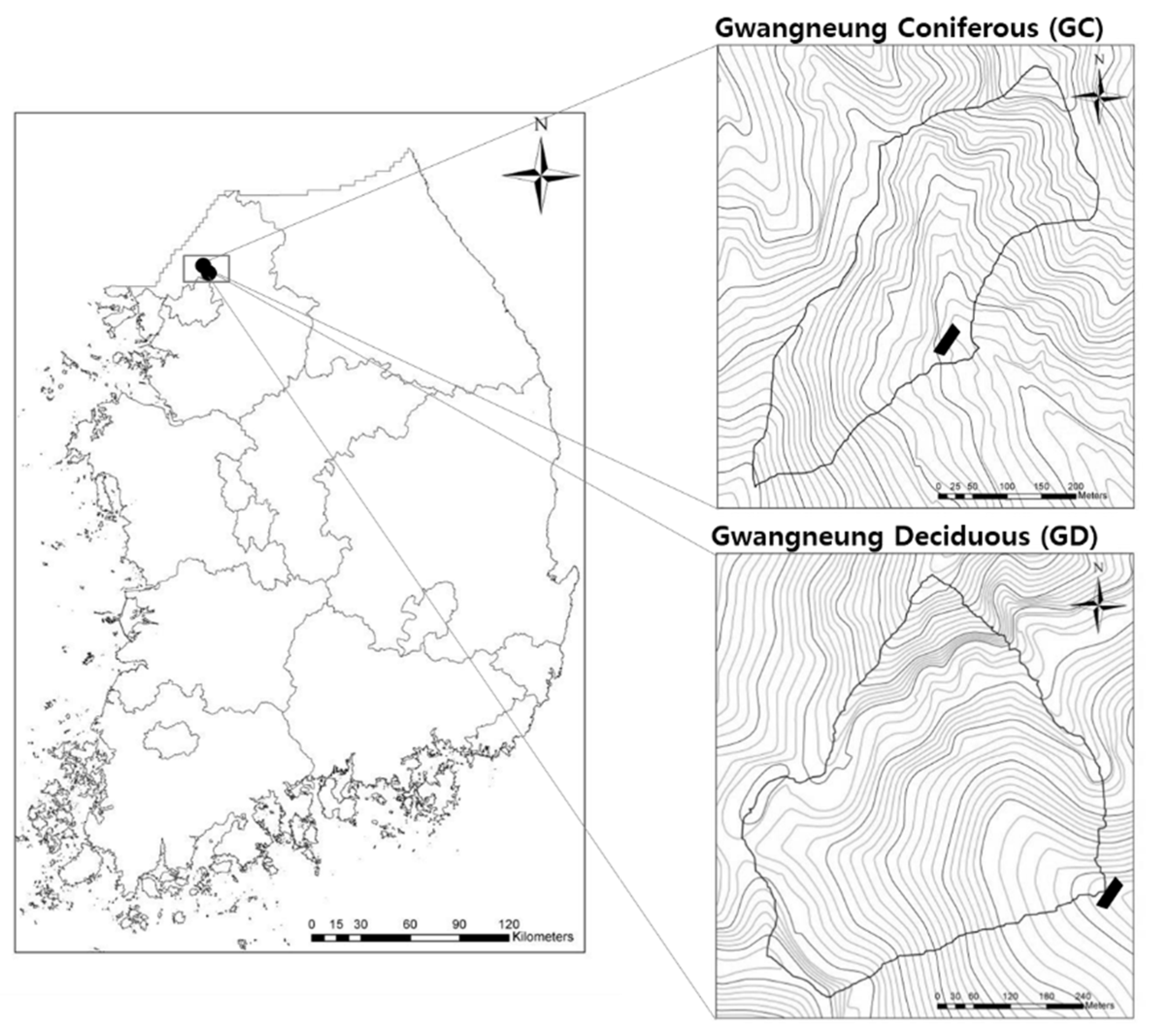
The study sites were two small forest catchments located in the National Experimental Forests in Pochun, Gyeonggi-do, South Korea: the Gwangneung coniferous forest (GC) catchment and the Gwangneung deciduous forest (GD) catchments (Figure 1). The GC catchment has an area of 13 ha and is covered with 30–60 cm thick sandy loam soil on the bed rock of granite gneiss (Table 1). The forests are mainly composed of Pinus koraiensis and Abies holophylla planted in 1976. The GD catchment has an area of 22 ha, and the soil conditions are similar to those of the GC catchment. In the GD catchment, natural old matured oak species and Larix kaempferi at almost 60 years old are preponderant. The mean annual precipitation is about 1502 mm and the mean annual temperature is about 11.2 °C in both catchments. Both catchments are close to each other—within 1 km distance—and so they are similar in terms of geology and climate, except for topography and forest conditions. The National Institute of Forest Science (NIFoS) has been collecting long-term rainfall-runoff data since 1980 at the streamflow gauging stations with a sharp-crested triangular (120°) weir installed in the outlets of both catchments. In this study, daily rainfall and runoff data collected from both catchments from 1982 to 2011 were used.
2.2. Determination of Recession Period
It is important to select appropriate recession periods from the streamflow hydrograph for baseflow recession analysis [9]. Runoff characteristics of forest catchments vary widely depending on the generations and compositions of direct runoff and baseflow [17], and so it is difficult to accurately understand these processes [11]. In other words, the point at which the direct runoff ends and where all runoff is baseflow should be carefully determined. White and Sloto [18] explained the point where direct runoff ends as a function of catchment area. In some cases, two days from the time of peak flow occurrence were excluded in the analysis because direct runoff is considered to be dominant during those periods [9]. Arnold et al. [12] and Cheng et al. [6] excluded two days from the time of peak flow occurrence for normal rainfall events and five days for heavy rainfall events. In addition, Vogel and Kroll [13] set the period from the point of time when the three-day moving average decreased to the point of time of increase on the time serial discharge data as a recession period.
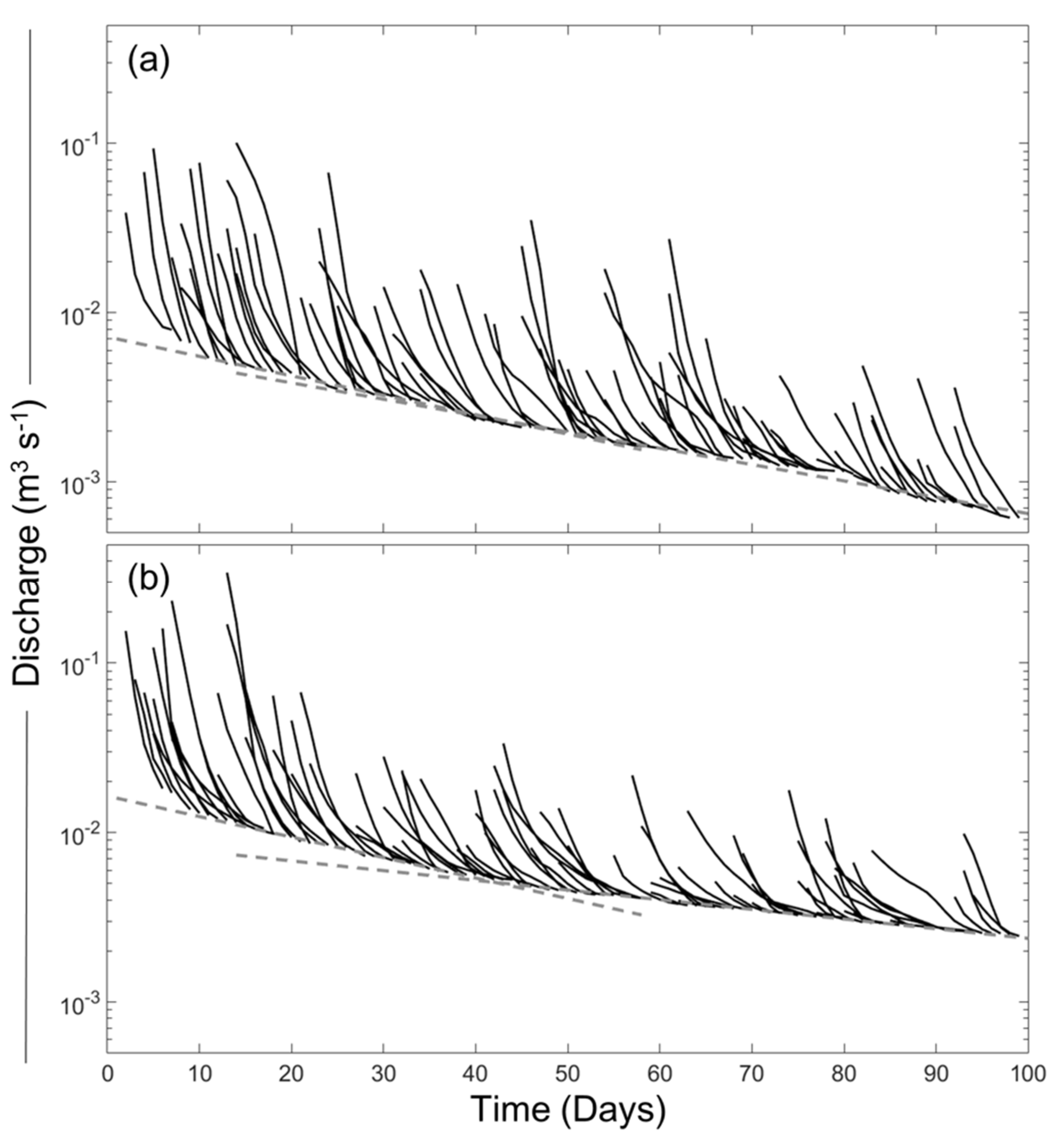
In this study, winter season data were excluded in determining recession periods due to freezing streamflow [19]. Also, during the dry periods, periods having at least eight consecutive days were selected as recession periods [6,7,14,15]. The point from two days after the time of peak flow occurrence was set as the point at which the direct runoff ends, given the findings of previous studies and the size of the catchment area. Thus, the streamflow hydrograph for periods from the point of direct runoff ending until just before the next rainfall event was extracted as a recession curve (Figure 2).
2.3. Estimation Methods for Baseflow Recession Constant
2.3.1. Theory of the Estimation of the Recession Constant
Previous research based on empirical phenomena and hydraulic theories have described the recession characteristic as the following [6,12,19,20]:
where is the baseflow after days (); is initial discharge at any time (); k is the mean residence time in days, which indicates the average time required for infiltrated water to pass the aquifer; is the recession constant, which is equivalent to . Equation (1) assumes the single linear reservoir ( where S is the volume of water stored and 86,400 is units conversion coefficient (s/day)), and it implies that the change in the baseflow over time considers the relationship between S and Q (). Several previous researchers have suggested the non-linearity of recession for a single linear reservoir [21,22]. However, considering its simplicity and practicality, Equation (1) is still often used [6,11,15]. In addition, as an equivalent to K is often applied, as shown in Equation (2). This implies that the baseflow consistently decreases at a constant rate during the recession period, and the recession constant accounts for most of the baseflow recession characteristics. Since the recession constant varies widely due to geographical, seasonal, and environmental influences, it is necessary to confirm the major trends with long-term streamflow data [9,23,24]. Six methods based on Equations (1) and (2) were used to estimate the recession constant.
2.3.2. Matching Strip Method (MS)
The matching strip method (MS) estimates the master recession curve by plotting all the recession curves in a semi-logarithmic graph [4,25]. Recession curves are added and moved horizontally until the master baseflow recession curve includes most of the recession curves’ tail ends [10]. This method allows the researcher to analyze recession characteristics by directly checking the master recession curve. However, it requires more long-term data than other methods, and results are different depending on the analyzer, because the master recession curve is drawn by the eye: the researcher’s subjective interpretation is required [6,10,11,26].
2.3.3. Correlation Method (CE, CR)
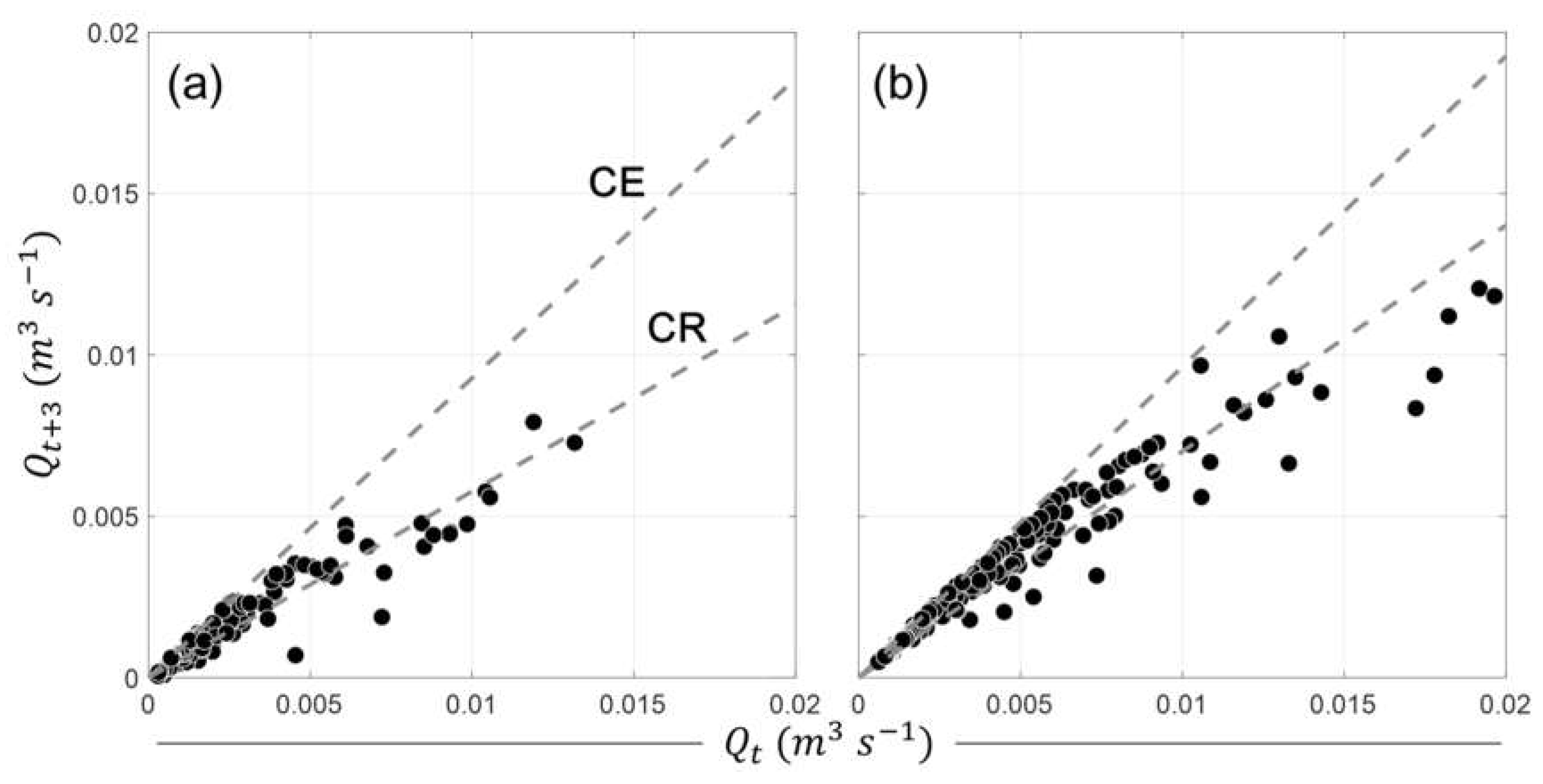
The correlation method is based on the reduced ratio during the same time interval [10,11]. For this, the discharge at any point in the recession curve and the discharge after days are plotted together as and -axis values, respectively. With this hypothesis, if the discharge at any one point is 0, the discharge after days is also 0; all the points in the graph and the origin are connected as a straight line [9]. The recession constant is determined through an enveloped line (CE: correlation method enveloped line) or a regression line (CR: correlation method regression line). The following equation is used to estimate the recession constant:
CE is the steepest slope on the graph and calculates the baseflow recession constant based on the smallest decrease record of time. The larger the time lag interval , the more accurate the value of the recession constant. However, in this case, CE needs longer periods of data [10]. In this study, a three-day lag interval was used.
2.3.4. Cheng Method (CH)
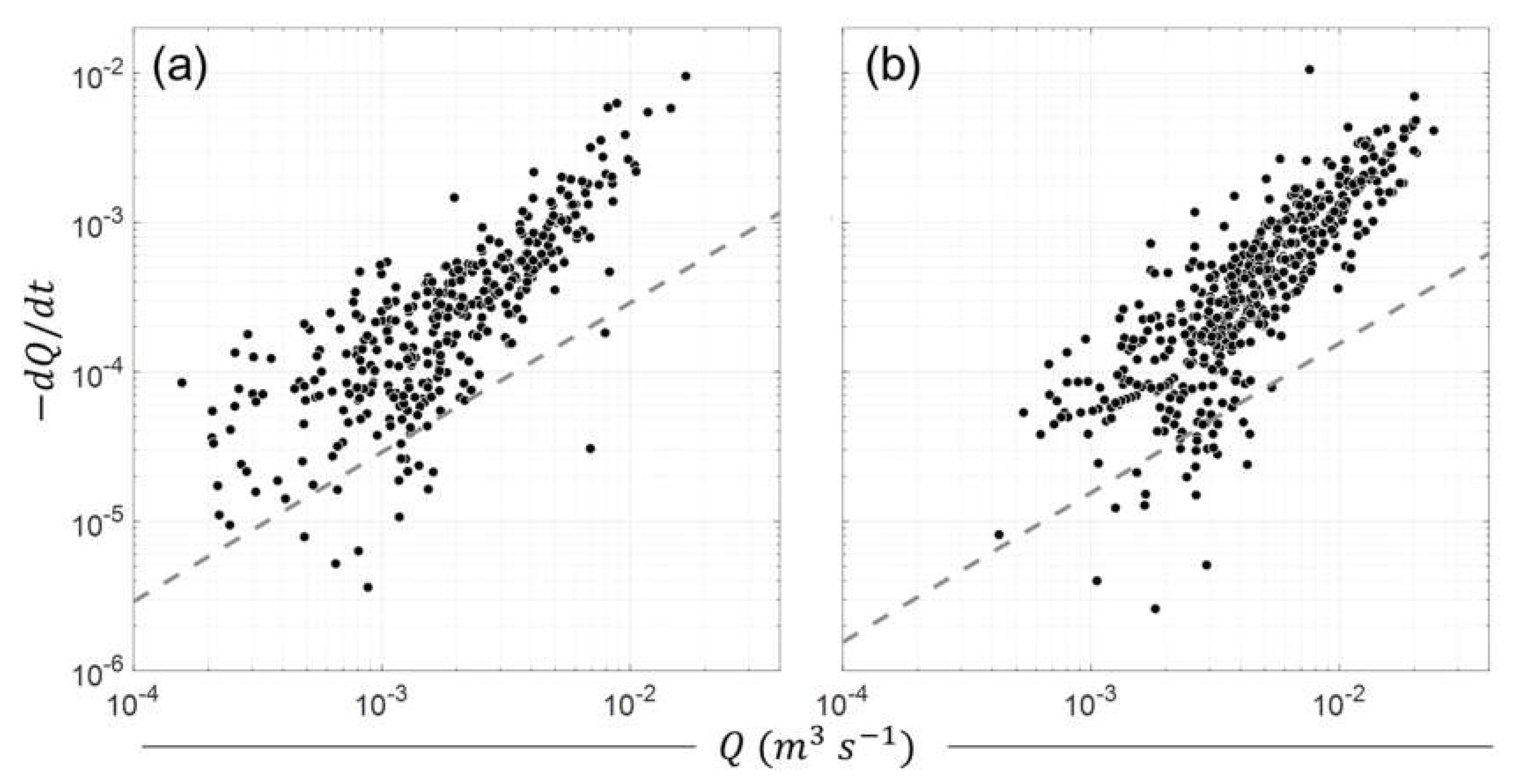
As an automatic algorithm for calculating recession constants, the automatic baseflow identification technique introduced by Cheng et al. [6] was used. The Cheng method (CH) has nine criteria that are used to select the pure baseflows from streamflow hydrograph. It calculates the recession constant from the relationship between the discharge of pure baseflow data () and the value of the recession slope (). The recession slope and corresponding flow have linear relationships, as shown in Equation (4), and the solution to this differential equation is Equation (1).
2.3.5. AR(1) Model
The autoregressive (AR) model explains the discharge at one point from a previous discharge in terms of the relationship between a discharge at one point and a discharge just before one point (AR(1) model) [27]. AR(1) is calculated using Equation (5) and adds the error term to Equation (1).
where is the mean daily streamflow on day in the th recession curve, is AR(1)’s recession constant of the th recession curve, and is the error on day in the th recession curve derived from the streamflow measurement or the model itself. is an independent and normally distributed error that has a zero mean and constant variance. In this study, the mean value of the recession constants calculated from the AR(1) model was set to represent the recession constant of one forest catchment.
2.3.6. Vogel and Kroll Method (VK)
When the streamflow is linearly related to the basin storage, Vogel and Kroll [14] calculated the recession constant with model error additives in log space. The baseflow recession constant is determined using the least squares method as follows:
where is the discharge after t days and m is the total number of two consecutive days streamflow pairs and at each catchment.
2.3.7. Validation Testing
In order to verify the validity of the six recession constant estimation methods (MS, CE, CR, CH, AR(1), and VK), we randomly selected and extracted three non-consecutive years of streamflow data in GC and GD. After calculating the recession constant from the remaining 27 years’ data, the validity was verified by comparing the measured discharge and the estimated discharge. As the evaluation criteria, root mean square error (RMSE) and measuring efficiency (ME) were calculated.
where is the measured discharge in the recession period, is the estimated discharge from the baseflow recession constant, and is the total number of independent recession series.
The validity of the recession constant was also verified by comparing the baseflow index (BFI), which is the ratio of baseflow to total streamflow, with previous studies. The baseflow was separated from the streamflow hydrograph with the recession constant. In order to separate the baseflow from the long-term streamflow data, with about 30 years of records, digital filtering, which separated the baseflow with an automated algorithm, was used [3,20,28]. In many digital filtering methods, the filter introduced by Eckhardt [28] was selected, as it describes forest catchment characteristics well.
where is the baseflow on day (), is the recession constant, and is the streamflow on day (). In perennial streams and porous aquifers, as found in the GC and GD forest catchments, a value of 0.8 was suggested [28].
3. Results
3.1. Rainfall-Runoff Characteristics in GC and GD Catchments
The rainfall-runoff characteristics of the GC and the GD catchments from 1982 to 2011 are presented in Table 2. Since daily streamflow data were used, the rainfall intensities are presented on a daily basis. A total of 62 and 61 rainfall-runoff events were collected from the long-term data of the GC and GD catchments, respectively. The rainfall events in the GC and GD catchments showed large variations in rainfall amount and intensity. In the GC catchment, the rainfall amount and intensity varied from 6 to 234 mm, and 6 mm day−1 to 20 mm day−1, respectively. In the GD catchment, 5–224 mm rainfalls and 5–112 mm·day−1 rainfall intensities were measured. The maximum mean daily discharge was 0.03 in the GC and 0.05 in the GD. The maximum mean daily discharge was estimated to be 1.7 times larger in the GD than the GC, which is thought to be due to the 1.6-fold larger catchment area of the GD.
3.2. Recession Constant Calculated by Six Estimation Methods
The 27-year recession constants (RC) and retention constants (mean residence time, k) of the GC and GD catchments, calculated by the six different methods, were estimated as follows (Table 3). First, using the matching strip method, the tangentization of the tail ends of the recession curves is shown in Figure 3. All recession curves have two tangents, as described by Rivera-Ramirez et al. [9]. It is because the linear reservoir does not fully explain the recessions. The recession constant calculated by the matching strip method was the largest among the other six methods.
The CE line and CR line were estimated from the correlation method, as shown in Figure 4. All the points in Figure 4 were located below the 1:1 line because they exist within the recession period. The recession constant obtained using CE, which represents the least reduced situation, was larger than that of CR. The CH method is shown in Figure 5, which defines the pure baseflow situation and shows the relationship between and . The dashed line is the fifth percentile value of each slope and has the value of a reciprocal of the recession constant. Both the AR(1) and VK method were estimated using the least-square method.
In the GC and GD catchments, MS, CE, and CH showed similar values, and CR, AR(1), and VK showed similar values. The recession constants and the k values that represent the mean residence time of the former group were smaller than the latter group. Consequentially, in both GC and GD catchments, MS had the largest recession constant and AR(1) the smallest recession constant.
3.3. Validation of the Six Methods
The root mean square error (RMSE) and measuring efficiency (ME) of each method were calculated to confirm the validity (Table 3). Based on the initial discharge of each recession curve, Equation (1) was applied to predict the baseflow. For calculating RMSE and ME, streamflow data for three non-consecutive years were used, except for the 27-year data that were used to estimate the representative baseflow recession constant.
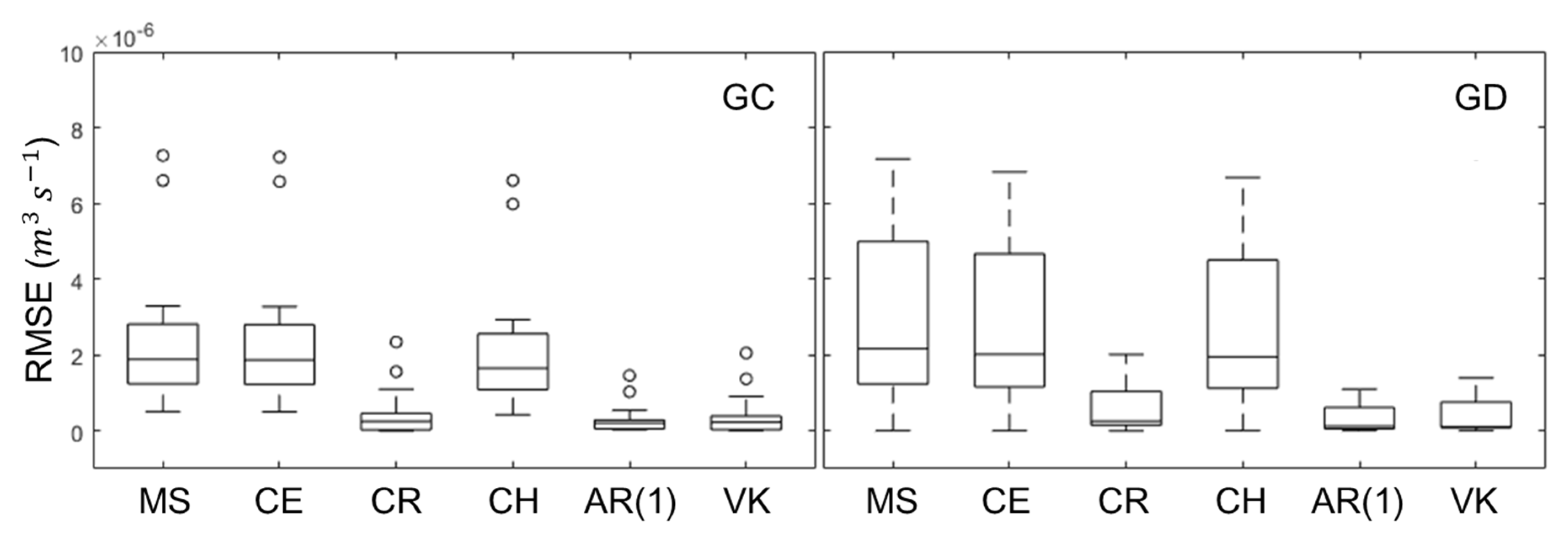
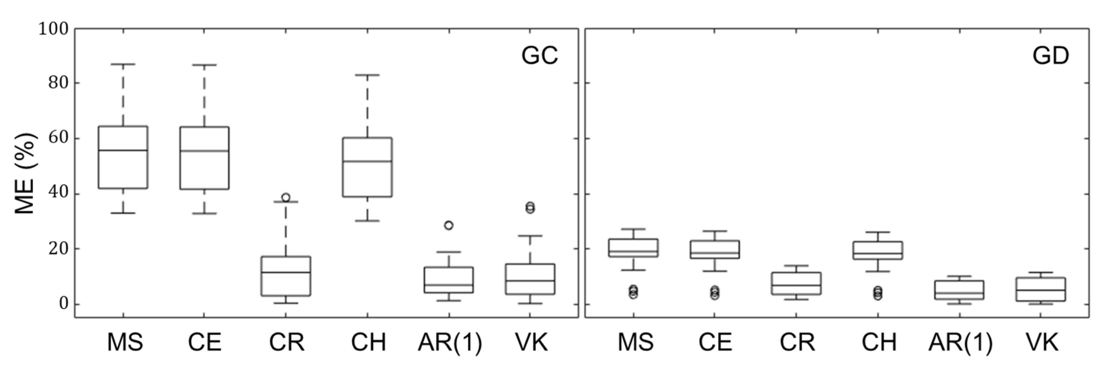
The RMSE and ME of MS, CR, and CH were the same and those of CR, AR(1), and VK were also equal, but the RMSE and ME of MS, CR, and CH were higher than those of CR, AR(1), and VK in the GC and GD catchments (Tukey’s test, p < 0.05; Figure 6 and Figure 7). The differences in RMSE values were double and the differences in ME were three- to six-fold. This means that baseflow prediction errors are larger when MS, CR, and CH are used.
There were differences between RMSE and ME for each method, but there were also differences between the GC and GD catchments. All RMSEs, which were calculated using six different methods, of the GD catchment were larger than those of the GC catchment. However, the measuring efficiencies of GD were smaller than those of the GC catchment. Thus, the six analytical methods worked better for the GD catchment than the GC.
Table 4 summarizes the BFI after separating the baseflow from the streamflow hydrograph using the six recession constant estimation methods. The lowest BFI was obtained when the MS recession constant was applied. BFI was 0.45 in the GC catchment and 0.48 in the GD catchment. On the other hand, the highest BFI was calculated when AR(1) was applied for estimating the recession constant. In this case, BFI was 0.69 in the GC catchment and 0.67 in the GD catchment. When applying the Eckhardt filter to separate baseflow, a smaller recession constant resulted in a larger BFI value, as applied in the same hydrograph.
4. Discussion
4.1. Differences between GC and GD Catchments
The RMSEs of the six analytical methods in the GD catchment were larger than those in the GC catchment, which could have been caused by the GD catchment area being 1.7 times larger. Because the GD catchment has the larger area, it discharges more streamflow. This resulted in a larger RMSE. However, the measuring efficiencies of the six methods in the GD catchment were smaller than those of the GC catchment. This result means that the six methods, assuming a linear reservoir, work better in the natural deciduous forest catchment. The GD catchment is natural forest that is more than 60 years old, whereas the GC catchment is an artificial forest planted in 1974. Since the GD catchment has been stabilized for a long time, this catchment may be better suited to the six analytical methods with linear reservoir assumption.
Recession characteristics are affected by both climatic and topographic factors [2]. However, since the GC and GD catchments have the same climatic characteristics, it can be assumed that the difference between topographic factors led to the larger recession constant of the GD catchment. The GD and GC catchments have the same geological characteristics, such as soil texture, soil depth, and bed rock, but different catchment shapes (Figure 1). Catchment elongation, which represents the catchment shape, was negatively correlated with the recession constant [29]. This means that the closer the catchment shape is to the shape of a circle, the smaller the derived recession constant is. According to this, since the GD catchment has a larger catchment elongation value, the recession constant of the GD catchment should be smaller. However, the recession constant of the GD catchment was larger than the GC catchment. Therefore, it is considered that there is another factor affecting the recession constant other than the catchment shape.
In addition to topographical factor, the main difference between the GD and GC catchments is forest cover. The GD catchment is covered by natural old deciduous forests and the GC catchment is covered by artificially planted coniferous forests with high tree density. The initial tree density at the time of planting was 3000 trees/ha, but is now about 1000–1200 trees/ha. With the same rainfall, more streamflow discharges from natural old deciduous forests because of the smaller evapotranspiration that occurs compared with coniferous forests [30,31]. The main factor influencing the recession characteristics was the evapotranspiration derived by different forest cover. When calculating the evapotranspiration ratio from the runoff ratio based on the water balance method, the GC catchment was 39% and GD was 33%. Thus, the GC catchment has a larger evapotranspiration per unit area than GD. This is the same as the result obtained by Choi [32], who previously studied the same GC and GD catchments and found different evapotranspiration values of each catchment. Richard [22] and Wittenberg [7] noted that evapotranspiration effects the recession constant and they found that the more evapotranspiration occurs, the smaller the calculated recession constant. This occurs because as more evapotranspiration occurs, plant root uptake increases, resulting in a small recession constant. Consequently, multiple factors, such as tree density, leaf area index, and forest stand age, caused a difference in the volume of evapotranspiration. Greater evapotranspiration in the GC catchment results in a smaller recession constant.
4.2. Different Recession Constants of the Six Estimation Methods
Recession constants calculated using MS, CE, and CH were similar at both GC and GD catchments. CR, AR(1), and VK were similar to each other. It was confirmed that the recession constants of MS, CE, and CH were larger than those of CR, AR(1), and VK.
The different mechanisms used by each method for estimating the recession constant cased the recession constant values to be different. MS estimates the recession constant around the tendency of the tail end parts of the recession curves. In addition, the lowest recession situation of all recession curves was determined using CE. CH considers the pure baseflow situation from the nine criteria and then calculates the fifth percentile of the recession rate as the representative recession constant of one catchment. In other words, the methods above derive the recession constant around the lower recession situations without considering most tendencies in recession curves. Therefore, these methods provide a somewhat larger the baseflow recession constant.
Conversely, the CR, AR(1), and VK methods estimate the recession constant by considering all baseflows in the recession curves. Additionally, we confirmed this finding when comparing the measured and calculated recession (Figure 8). First, CR calculates the representative recession constant through the regression line of the recession rates. The AR(1) and VK methods assume a linear reservoir and then estimate the recession constant by estimating coefficients that are fitted to the governor equation. These methods are the same in that the recession constants of all recession curves are obtained based on the least squares method, although their approaches for solving are different. Thus, the CR, AR(1), and VK methods calculate smaller baseflow recession constants than MS, CE, and CH in both GC and GD catchments.
4.3. Applicability Assessment
Among the six methods, the baseflow prediction rates of CR, AR(1), and VK methods were higher than those of the other three methods. This suggests that the MS, CE, and CH methods are overestimating the baseflow recession constant in the study area. In general, the baseflow recession constant ranged from 0.75 to 0.95 [14,33]. The recession constants of CR, AR(1), and VK methods fell within this range, whereas the recession constants of MS, CE, and CH were larger.
The recession constants of MS, CE, and CH also underestimated the baseflow index. The baseflow index in the forest catchment is generally in the range of 58 to 78% [28,34]. When the baseflow separation was conducted with the recession constants of CR, AR(1), and VK as the filter parameters, the range of BFI was 0.64 to 0.69, which is within the range of the preceding research. The BFI ranges of MS, CE, and CH, however, were 0.45 to 0.50, which do not fall within the previous study range, and so these methods cannot reasonably explain the baseflow of small forest catchments.
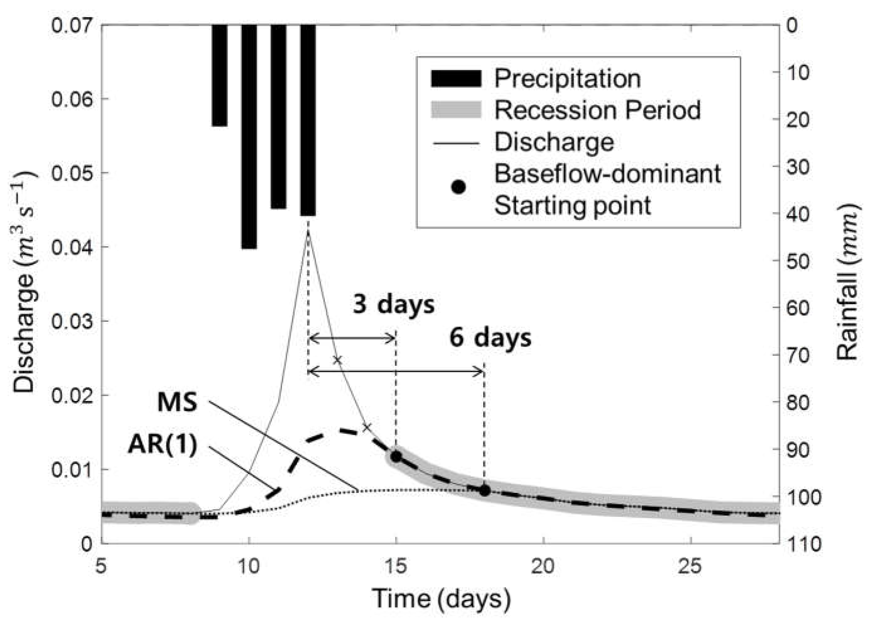
Baseflow is the streamflow involving soil moisture or aquifer water, which is slower than the direct runoff [35]. Hewlett and Hibbert [16] noted that in forests with trees and porous soils, most of the rainfall is first stored in the soil layer before flowing. In other words, due to the watershed conservation function of forests, most of the runoff characteristics of the forest catchment can be explained as a baseflow process, which should not be confused with groundwater flow [2]. Therefore, in the GC and GD catchments, most of the streamflow starting three days after the peak flow was the baseflow. In the case of the CR, AR(1), and VK methods, the anticipated baseflow starting two to three days after the peak flow reasonably explained most of the corresponding streamflow (Figure 9). Conversely, when the streamflow was separated by the recession constants calculated using MS, CE and CH, the anticipated baseflow explained the corresponding streamflow 6–10 days after the peak flow. Taken together, MS, CE, and CH seem to explain the characteristics of the groundwater flow better in forest catchments, which is slower than baseflow. That is, using use the CR, AR(1), and VK to estimate the baseflow recession constant in small forest catchments would be more reasonable.
5. Conclusions
This study was conducted to assess the applicability of the recession constant estimating methods in small forest catchments. For this purpose, long-term streamflow data (1982–2011) of a natural old deciduous forest (GD) and a planted coniferous forest (GC) catchment in Gwangneung were used to calculate the recession constants with each method.
Six recession constant estimation methods were selected because these have been used in many previous studies. The recession constants of the GC and GD catchments were calculated using these methods. All six methods yielded larger recession constants in the GD catchment. The GC and GD catchments have the same climatic conditions and geological features, but they have different catchment shapes and forest cover. Previous studies have noted that the larger the catchment elongation, which is the factor representing the catchment shape, the smaller the recession constant. However, the GD catchment, which had a larger catchment elongation value, had the larger recession constants. We inferred that the difference in forest cover had a greater effect than the catchment shape on the difference between the recession constants. Many previous studies have suggested that different infiltration rates and evapotranspiration rates are observed according to the forest cover, even under the same rain conditions. Similar to previous studies in which the deciduous forest catchment exhibited lower evapotranspiration rates than the coniferous forests, we confirmed that the GD catchment has a larger recession constant.
Validation testing was conducted to assess the applicability of the six recession constant estimation methods. Recessions were predicted from the recession constants derived from each method, and the RMSE and ME of each method were calculated. As a result, the CR, AR(1), and VK methods had relatively low RMSE and ME compared with MS, CE, and CH. Conversely, the recession constants of CR, AR(1), and VK methods were within the range of previous studies. The BFIs calculated using these methods were also similar to those of previous studies. When MS, CR, and CH were used for the baseflow separation, the baseflow was able to explain most of the streamflow starting from 6–10 days after rainfall. These results suggest that these methods are not suitable for explaining baseflow characteristics of small forest catchments.
This study demonstrated that it is more reasonable to use the CR, AR(1), and VK methods to analyze baseflow recession characteristics in small forest catchments. However, all of these methods require the reasonable selection of recession periods in streamflow hydrographs. Thus, when a different method is used to measure the baseflow characteristics other than these six methods to determine the baseflow-dominant period, such as tracer-based methods, a more reasonable analysis of forest recession characteristics can be achieved.
Author Contributions
Conceptualization, H.Y. and H.T.C.; Methodology, H.Y.; Software, H.Y.; Validation, H.Y. and H.T.C.; Formal Analysis, H.Y.; Investigation, H.T.C. and H.L.; Resources, H.T.C. and H.L.; Data Curation, H.T.C. and H.L.; Writing-Original Draft Preparation, H.Y. and H.L.; Writing-Review and Editing, H.Y. and H.T.C.; Visualization, H.Y.; Supervision, H.T.C.; Project Administration, H.T.C. and H.L.; Funding Acquisition, H.T.C.
Funding
This research received no external funding.
Conflicts of Interest
The authors declare no conflict of interest.
References
- Cherkauer, D.S.; Ansari, S.A. Estimating ground water recharge from topography, hydrogeology, and land cover. Groundwater. 2005, 43, 102–112. [Google Scholar] [CrossRef]
- Price, K. Effects of watershed topography, soils, land use, and climate on baseflow hydrology in humid regions: A review. Prog. Phys. Geogr. Earth Environ. 2011, 35, 465–492. [Google Scholar] [CrossRef]
- Lim, K.J.; Engel, B.A.; Tang, Z.; Choi, J.; Kim, K.S.; Muthukrishnan, S.; Tripathy, D. Automated web GIS based hydrograph analysis tool, WHAT. J. Am. Water Resour. Assoc. 2005, 41, 1407–1416. [Google Scholar] [CrossRef]
- Smakhtin, V.U. Low flow hydrology: A review. J. Hydrol. 2001, 240, 147–186. [Google Scholar] [CrossRef]
- Hoos, A.B. Recharge Rates and Aquifer Hydraulic Characteristics for Selected Drainage Basins in Middle and East Tennessee; U.S. Geological Survey: Reston, VA, USA, 1990.
- Cheng, L.; Zhang, L.; Brutsaert, W. Automated selection of pure base flows from regular daily streamflow data: Objective algorithm. J. Hydrol. Eng. 2016, 21, 06016008. [Google Scholar] [CrossRef]
- Wittenberg, H. Effects of season and man-made changes on baseflow and flow recession: Case studies. Hydrol. Process. 2003, 17, 2113–2123. [Google Scholar] [CrossRef]
- Posavec, K.; Parlov, J.; Nakić, Z. Fully automated objective-based method for master recession curve separation. Groundwater 2010, 48, 598–603. [Google Scholar] [CrossRef] [PubMed]
- Rivera-Ramirez, H.D.; Warner, G.S.; Scatena, F.N. Prediction of master recession curves and baseflow recessions in the Luquillo Mountains of Puerto Rico. J. Am. Water Resour. Assoc. 2002, 38, 693–704. [Google Scholar] [CrossRef]
- Nathan, R.; McMahon, T. Evaluation of automated techniques for base flow and recession analyses. Water Resour. Res. 1990, 26, 1465–1473. [Google Scholar] [CrossRef]
- Sujono, J.; Shikasho, S.; Hiramatsu, K. A comparison of techniques for hydrograph recession analysis. Hydrol. Process. 2004, 18, 403–413. [Google Scholar] [CrossRef]
- Arnold, J.; Allen, P.; Muttiah, R.; Bernhardt, G. Automated base flow separation and recession analysis techniques. Groundwater 1995, 33, 1010–1018. [Google Scholar] [CrossRef]
- Vogel, R.M.; Kroll, C.N. Estimation of baseflow recession constants. Water Resour. Manag. 1996, 10, 303–320. [Google Scholar] [CrossRef]
- Vogel, R.M.; Kroll, C.N. Regional geohydrologic-geomorphic relationships for the estimation of low-flow statistics. Water Resour. Res. 1992, 28, 2451–2458. [Google Scholar] [CrossRef]
- Fiorotto, V.; Caroni, E. A new approach to master recession curve analysis. Hydrol. Sci. J. 2013, 58, 966–975. [Google Scholar] [CrossRef] [Green Version]
- Hewlett, J.D.; Hibbert, A.R. Factors affecting the response of small watersheds to precipitation in humid areas. For. Hydrol. 1967, 1, 275–290. [Google Scholar]
- Singh, K.P.; Stall, J.B. Derivation of base flow recession curves and parameters. Water Resour. Res. 1971, 7, 292–303. [Google Scholar] [CrossRef]
- White, K.E.; Sloto, R.A. Base-Flow Frequency Characteristics of Selected Pennsylvania Streams; U.S. Geological Survey: Reston, VA, USA, 1990.
- Brandes, D.; Hoffmann, J.G.; Mangarillo, J.T. Base flow recession rates, low flows, and hydrologic features of small watersheds in Pennsylvania, USA. J. Am. Water Resour. Assoc. 2005, 41, 1177–1186. [Google Scholar] [CrossRef]
- Zhang, J.; Zhang, Y.; Song, J.; Cheng, L. Evaluating relative merits of four baseflow separation methods in Eastern Australia. J. Hydrol. 2017, 549, 252–263. [Google Scholar] [CrossRef]
- Chapman, T.G. Modelling stream recession flows. Environ. Modell. Softw. 2003, 18, 683–692. [Google Scholar] [CrossRef]
- Weisman, R.N. The effect of evapotranspiration on streamflow recession. Hydrol. Sci. Bull. 1977, 22, 371–377. [Google Scholar] [CrossRef]
- Lamb, R.; Beven, K. Using interactive recession curve analysis to specify a general catchment storage model. Hydrol. Earth Syst. Sci. 1997, 1, 101–113. [Google Scholar] [CrossRef] [Green Version]
- Wang, D.; Cai, X. Detecting human interferences to low flows through base flow recession analysis. Water Resour. Res. 2009, 45, W07426. [Google Scholar] [CrossRef]
- Lee, I.S.; Lee, H.H. Analysis of secular changes in the hydrological characteristics of a small forested watershed using a baseflow recession curve. J. Korean For. Soc. 2014, 103, 383–391. [Google Scholar] [CrossRef]
- Rutledge, A. Computer Programs for Describing the Recession of Ground-Water Discharge and for Estimating Mean Ground-Water Recharge and Discharge from Streamflow Records; U.S. Geological Survey: Reston, VA, USA, 1998.
- Box, G.E.P.; Jenkins, G.M.; Reinsel, G.C.; Ljung, G.M. Time series analysis: Forecasting and control; John Wiley & Sons, Inc.: Hoboken, NJ, USA, 1970. [Google Scholar]
- Eckhardt, K. How to construct recursive digital filters for baseflow separation. Hydrol. Process. 2005, 19, 507–515. [Google Scholar] [CrossRef]
- Peña-Arancibia, J.; Van Dijk, A.; Mulligan, M.; Bruijnzeel, L.A. The role of climatic and terrain attributes in estimating baseflow recession in tropical catchments. Hydrol. Earth Syst. Sci. 2010, 14, 2193–2205. [Google Scholar] [CrossRef] [Green Version]
- Komatsu, H.; Kume, T.; Otsuki, K. The effect of converting a native broad-leaved forest to a coniferous plantation forest on annual water yield: A paired-catchment study in northern Japan. For. Ecol. Manage. 2008, 255, 880–886. [Google Scholar] [CrossRef]
- Swank, W.T.; Douglass, J.E. Streamflow greatly reduced by converting deciduous hardwood stands to pine. Science 1974, 185, 857–859. [Google Scholar] [CrossRef] [PubMed]
- Choi, H.T. Effect of forest growth and thinning on the long-term water balance in a coniferous forest. Korean Soc. Agric. For. Meteorol. 2011, 4, 157–164. [Google Scholar] [CrossRef]
- Lee, J.C.; Park, U.K.; Jung, J.S. A study on estimation of recession constant in base flow. J. Korean Soc. Environ. Technol. 2001, 2, 7–15. [Google Scholar]
- Jeong, Y.H.; Kim, K.H.; Chung, C.G.; Jun, J.H.; Yoo, J.Y. Effects of forest fire on the quantities and qualities of the streamwater in small forest catchments. J. Korean For. Soc. 2004, 93, 446–452. [Google Scholar]
- Sklash, M.G.; Farvolden, R.N. The role of groundwater in storm runoff. J. Hydrol. 1979, 43, 45–65. [Google Scholar] [CrossRef]
Figure 1.
Location of the study sites.

Figure 2.
Determination of the recession periods from the Gwangneung deciduous (GD) catchment rainfall-runoff data. Two days after peak flow were excluded and recessions were chosen as being over eight days in length. The hydrograph was performed for periods at least eight consecutive days from the point at which two days passed after the peak flow until just before the next rainfall event was extracted. is the initial discharge and is generally the starting point of the recession discharge.

Figure 3.
Master recession curves derived from the matching strip method at the (a) Gwangneung coniferous (GC) and (b) GD catchments. Master recession curves have two tangents because the linear reservoir does not fully explain the recessions.
Figure 3.
Master recession curves derived from the matching strip method at the (a) Gwangneung coniferous (GC) and (b) GD catchments. Master recession curves have two tangents because the linear reservoir does not fully explain the recessions.

Figure 4.
Recession constants obtained with the correlation method at the (a) GC and (b) GD catchments. The higher gradient line is the correlation enveloped line (CE) and the lower gradient line is the correlation regression line (CR).
Figure 4.
Recession constants obtained with the correlation method at the (a) GC and (b) GD catchments. The higher gradient line is the correlation enveloped line (CE) and the lower gradient line is the correlation regression line (CR).

Figure 5.
Relationship between the discharge and recession slope that were passed through the nine required criteria for CH [6] at the (a) GC and (b) GD catchments. The fifth percentile enveloped line has the gradient of the reciprocal of the recession constant.
Figure 5.
Relationship between the discharge and recession slope that were passed through the nine required criteria for CH [6] at the (a) GC and (b) GD catchments. The fifth percentile enveloped line has the gradient of the reciprocal of the recession constant.

Figure 6.
Root mean square error (RMSE) of the six methods in the GC and GD catchments.

Figure 7.
Measuring efficiencies (ME) of six methods in the GC and GD catchments.

Figure 8.
The real measured recession with calculated recessions by six estimation methods. The MS, CE, and CH methods tend to overestimate the recessions, whereas the CR, AR (1), and VK methods described the recessions relatively well.
Figure 8.
The real measured recession with calculated recessions by six estimation methods. The MS, CE, and CH methods tend to overestimate the recessions, whereas the CR, AR (1), and VK methods described the recessions relatively well.

Figure 9.
Baseflow separation with the Eckhardt filter [28] from the GD catchment rainfall-runoff data. The baseflow-dominant points where AR(1) model was used started two to three days after the peak flow, whereas points where MS was used stared 6–10 days after the peak flow.
Figure 9.
Baseflow separation with the Eckhardt filter [28] from the GD catchment rainfall-runoff data. The baseflow-dominant points where AR(1) model was used started two to three days after the peak flow, whereas points where MS was used stared 6–10 days after the peak flow.


Table 1.
Characteristics of the Gwangneung coniferous (GC) and Gwangneung deciduous (GD) forest catchments.
Table 1.
Characteristics of the Gwangneung coniferous (GC) and Gwangneung deciduous (GD) forest catchments.
| Catchment Characteristic | GC | GD |
|---|---|---|
| Catchment area (ha) | 13 | 22 |
| Elevation (m) | 160–290 | 280–470 |
| Bed rock | Granite gneiss | Granite gneiss |
| Soil depth (m) | 0.3–0.6 | 0.3–0.6 |
| Predominant species | Pinus koraiensis Abies holophylla | Oak species Larix kaempferi |
| Tree density (trees/ha) | 1400–1500 | 1000–1200 |
| Forest stand age (years) | 7–36 | 60–90 |
| Remarks | Planted in 1976 | Natural forest |
Table 2.
Rainfall-runoff characteristics of the study sites (1982–2011).
| Rainfall-Runoff Characteristic | GC | GD |
|---|---|---|
| Number of rainfall-runoff events | 62 | 61 |
| Rainfall (mm) | 49.12 ± 47.19 | 44.67 ± 37.59 |
| Rainfall intensity () | 28.31 ± 19.91 | 27.22 ± 18.25 |
| Peak flow () | 0.03 ± 0.10 | 0.05 ± 0.13 |
| Baseflow index, BFI | 0.73 ± 0.09 | 0.72 ± 0.12 |
| Runoff ratio (runoff/rainfall) | 0.61 | 0.67 |
| Recession constant, RC | 0.85 ± 0.08 | 0.92 ± 0.03 |
Note: Values indicate the mean SD, and Baseflow index (BFI) and recession constant (RC) were derived by AR(1) method.
Table 3.
Recession constants (RC), mean residence time (k), root mean square error (RMSE), and measuring efficiency (ME) of the GC and GD catchments.
Table 3.
Recession constants (RC), mean residence time (k), root mean square error (RMSE), and measuring efficiency (ME) of the GC and GD catchments.
| Calculate Method | GC | GD | ||||||
|---|---|---|---|---|---|---|---|---|
| RC | RMSE | ME | RC | RMSE | ME | |||
| MS | 0.9779 | 45 | 1.02 | 32.2 | 0.9875 | 80 | 1.86 | 16.2 |
| CE | 0.9775 | 44 | 1.00 | 32.1 | 0.9854 | 69 | 1.83 | 15.9 |
| CR | 0.8752 | 8 | 0.49 | 10.3 | 0.9406 | 16 | 1.30 | 8.6 |
| CH | 0.9708 | 34 | 0.97 | 32.5 | 0.9844 | 64 | 1.82 | 16.4 |
| AR(1) | 0.8480 | 6 | 0.41 | 5.3 | 0.9235 | 13 | 1.13 | 5.9 |
| VK | 0.8670 | 7 | 0.46 | 8.8 | 0.9298 | 14 | 1.19 | 6.9 |
Note: k is expressed in days, RMSE is expressed as , and ME is dimensionless (%).
Table 4.
Baseflow index (BFI) of the GC and GD catchments calculated using the six different baseflow recession constant estimation methods.
Table 4.
Baseflow index (BFI) of the GC and GD catchments calculated using the six different baseflow recession constant estimation methods.
| Catchment | MS | CE | CR | CH | AR(1) | VK |
|---|---|---|---|---|---|---|
| GC | 0.4484 | 0.4611 | 0.6664 | 0.4829 | 0.6898 | 0.6741 |
| GD | 0.4755 | 0.4916 | 0.6397 | 0.4984 | 0.6663 | 0.6574 |
© 2018 by the authors. Licensee MDPI, Basel, Switzerland. This article is an open access article distributed under the terms and conditions of the Creative Commons Attribution (CC BY) license (http://creativecommons.org/licenses/by/4.0/).
Share and Cite
MDPI and ACS Style
Yang, H.; Choi, H.T.; Lim, H. Applicability Assessment of Estimation Methods for Baseflow Recession Constants in Small Forest Catchments. Water 2018, 10, 1074. https://doi.org/10.3390/w10081074
AMA Style
Yang H, Choi HT, Lim H. Applicability Assessment of Estimation Methods for Baseflow Recession Constants in Small Forest Catchments. Water. 2018; 10(8):1074. https://doi.org/10.3390/w10081074
Chicago/Turabian StyleYang, Hyunje, Hyung Tae Choi, and Honggeun Lim. 2018. "Applicability Assessment of Estimation Methods for Baseflow Recession Constants in Small Forest Catchments" Water 10, no. 8: 1074. https://doi.org/10.3390/w10081074
Note that from the first issue of 2016, this journal uses article numbers instead of page numbers. See further details here.