Modeling Approach for Water-Quality Management to Control Pollution Concentration: A Case Study of Ravi River, Punjab, Pakistan


Graduate School of Water Resources, Sungkyunkwan University, 2066, Seobu-ru, Suwon-si 440746, Korea
*
Author to whom correspondence should be addressed.
Water 2018, 10(8), 1068; https://doi.org/10.3390/w10081068
Submission received: 25 June 2018
/
Revised: 7 August 2018
/
Accepted: 8 August 2018
/
Published: 10 August 2018
(This article belongs to the Section Water Quality and Contamination)
Abstract
:One of the challenging problems of Punjab, the most populous province of Pakistan, is the surface water-quality problem of the Ravi River, which flows through the main cities of the province. At present, the overall status of water quality is very polluted, primarily due to residential and industrial wastewater directly discharged into the Ravi River through a network of drains. Due to the poor quality of the water, the river ecosystem is not favorable for the aquatic and surrounding environment. Hence, management options are proposed to reduce pollution. Therefore, the study was formulated to identify the main sources of pollution along the Ravi River and their potential impact on the course of the river channel. In addition, the study applied a numerical model WASP 8.1 (Water Quality Simulation Program) to discover the best strategy for the improvement of water quality. Through the model simulation it was found that, if the flow at headwater and link canals is increased up to 50%, along with 75% improvement in the pollution concentration of drains through wastewater-treatment facilities, the water quality of the Ravi River can be improved up to an acceptable limit of water-quality standards.
1. Introduction
Urban development without sound strategies causes various environmental problems for several water resources, such as rivers, lakes, canal, and reservoirs [1,2,3,4]. Rapid urbanization and industrial growth multiplied the production of wastewater through effluent discharge. If wastewater goes in nearby streams without proper treatment, it causes various environmental issues for human beings and aquatic life [5,6]. In other words, urbanization without sustainable planning deteriorates the water ecosystem. Therefore, developed countries have implemented proper urban water-quality management plans by installing wastewater-treatment facilities at disposal sites. However, many cities in developing countries have been urbanized without such planning; untreated water generated from residential and industrial areas contaminate the receiving water ecosystem [7].
The uncontrolled disposal of various pollutants such as Biological Oxygen Demand (BOD), Total Dissolved Solids (TDS), Total Suspended Solids (TSS), Total Nitrogen (TN), and Total Phosphorus (TP) flowing into water bodies often causes various environmental issues, such as production of harmful algal blooms, eutrophication, death of aquatic life, decline of biodiversity, and ultimately gravely affecting human life [8]. The current water pollution threatens the sustainability of the river ecosystem and the urban area alongside the river. Therefore, it is direly needed to control the water-quality concentration up to an optimum level to conserve water ecology. Thus, many countries such as China, Malaysia, and Korea have installed wastewater-treatment plants alongside river streams to conserve water ecology [9]. In order to launch reliable water-quality management plans to conserve riverwater environments, the best management scenarios are necessary to be made, which are feasible and economical [8,10].
Previous research has been limited to assessment of observation and simulated data [7]. However, efficient management and planning require sound strategies by considering both current and future possible scenarios to keep the water ecosystem viable. Assessment of current conditions and management strategies for the Ravi River is proposed to discover alternative quality- and quantity-control options. The development of a water-quality management scenario requires a broad knowledge of present degradation causes and pollution sources for precise management solutions [7,11,12,13].
In recent years, water-quality modeling has been used for the assessment and management of environmental problems of urban water environments. Computer-based numerical models are more valuable than traditional manual monitoring, experimental, and empirical models in urban water-quality assessment and management [14,15]. A numerical model simulates the water-quality status of a river ecosystem for likely assessment and management scenarios throughout the course of the river channel [13,16].
With advances in computation and processing technology in the twenty-first century, a large number of substantial improvements have been made in the area of surface water-quality simulation tools that have led to the varieties of surface water-quality models. Currently, there are many water-quality models for strategy development and decision-making purposes for different types of water bodies. These models have been improving continuously based on the latest innovation and studies [17,18,19]. Recently, several water-quality models, such as the EFDC, TOMCAT, MIKE, PAMOLARE, BASINS, CAEDYM, Streeter-Phelps, AQUATOX, QUASAR, Water Quality Simulation Program (WASP), QUAL2E/K/Kw, and CE-QUAL/W-2 model have been constructed for simulating the status of the water quality of lakes, rivers, and estuaries worldwide [20,21,22,23]. However, a recent review study determined that, among these different publicly used commercial and open-source models, the WASP is one of the most suitable water-quality models for simulating the transport and fate of the pollutants in rivers and reservoirs [24].
The United States Environmental Protection Agency (USEPA) developed the WASP model for surface water-quality modeling [25]. With the advancement of different versions, the WASP model has been applied worldwide for simulation and assessment of surface-water pollution [26,27,28,29]. For example, it has been applied for local risk assessment of direct discharge of the pollution load into the Taipu River, China [30]. Recently, it was also applied for the eutrophication evaluation over the Taihu and Beihai Lakes, China [31]. Similarly, some other practical applications have been used globally to forecast the impacts of management strategies on ecosystems, water environments, and to measure pollution loads to establish sustainable planning [10,32,33].
This study simulates the longitudinal profile of different water-quality parameters along the course of the Ravi River channel, Punjab Province. Assessment of simulated water-quality profiles can be helpful in urban river water-quality evaluation and management planning. The study identifies major point sources, their pollution-loading shares, and overall shares of main cities along the section of Ravi River. Furthermore, this study also provides suitable scenario-based management strategies to control pollution concentration for improving the urban water ecosystem of the Punjab province, Pakistan.
2. Materials and Methods
2.1. Study Area
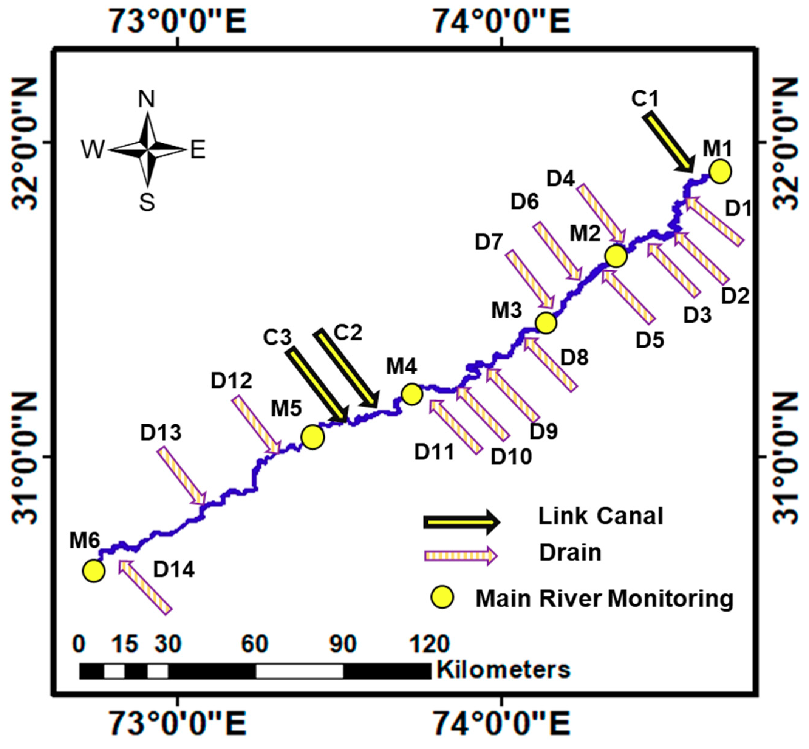
Punjab is the most populous province of Pakistan. The population of Pakistan is growing rapidly. The national census of 2017 recorded the population of Pakistan at about 210 million. The population of the Punjab province is about 110 million, nearly 53% of the entire residents [34,35,36]. The Ravi River basin is the transboundary basin between Pakistan and India and is one of the main rivers of the Indus System in the Punjab province. The river originates in the Himalayas region, flowing from northwest Himachal Pradesh, India to the southeast, in Punjab, Pakistan [37,38,39]. The river enters Pakistan near Jassar and meets with the river Chenab at Head Sidhnai. The study area lies between 30°50′5″ to 32°0′0″ N latitude and 72°50′0″ to 74°30′0″ E longitude (Figure 1). The Ravi River is the smallest river among five other rivers of the Indus basin system flowing in Pakistan.
The general altitude of the area is about 207 to 213 m above mean sea level. The total catchment area of the river basin is about 40,769 km2 [40]. The average annual flow near Mukesar, India is 267.5 m3/s [41]. The total length of the Ravi River, both in India and Pakistan, is about 720 km. The topography of the river course is almost flat, sloping from the north toward the southwest, with an average gradient of the slope being 1:3000. The surface soil layer is fine-grained fertile (alluvial soil) deposited by water flow over the bed of the river, while the underneath soil layer mostly consists of a mixture of clay, silt, and gravel. The region also possesses a huge variation in the temporal pattern of extreme climate, ranging from –1 °C to 46 °C. Throughout the year, short events of rainfall occur, especially in the months of July and August due to summer monsoons. The mean annual rainfall in the study region is about 620 mm. The relative humidity of the study region varies between 45% to 85% and average wind speed fluctuates from 0.1 to 1.6 m/s throughout the year [40,42].
A continuously growing population, high industrial development, and rapid urbanization without proper planning have resulted in the degradation of water quality of the Ravi River. In the Punjab province, the residential and industrial wastewater from almost every region is discharged into nearby drains, eventually flowing to nearby rivers. This has caused serious water pollution, human health problems, and eventually has posed serious problems for the environment. Residential, industrial, and agricultural waste contaminates the river with chemicals and pathogens that may cause eutrophication problems, threatening human and river environments. The main source of contamination of the Ravi River is wastewater drains that flow into the river. These drains carry the industrial and sewage wastewater of urban areas of the Lahore, Sheikhupura, Faisalabad, and Sahiwal districts. Many small drains join large drains and link canals and ultimately fall in the Ravi River [43,44,45]. The major drain and link canals that fall into segments of the Ravi River are the Mehmood Booti Drain (D1), Sukh Naher Drain (D2), Shad Bagh Drain (D3), Shahdara Town Pumping Station (D4), Forest Colony Pumping Station (D5), Farukhabad Drain (D6), Budha Ravi Drain (D7), Main Outfall Drain (D8), Gulshan-E-Ravi Drain (D9), Babu Sabu Drain (D10), Hudiara Drain (D11), Jaranwala Drain (D12), Samundari Drain (D13), Sukhwara Drain (D14), Marala Ravi Link Canal (C1), Upper Chenab Canal (C2), and Qadrabad Balloki Link Canal (C3).
2.2. Data Collection for Water-Quality Assessment.
For the better assessment of the current condition of river water quality, model calibration, and validation, 3 water-sampling events were conducted between April and May 2018 during the low-flow season (Tables S1–S3). A total of 6 samples were collected from the main stem of the Ravi River M1–M6, 14 stations’ data were collected from main drains before the confluence into the river, and 3 samples from link canals before confluence into the Ravi River (Table 1). Samples were collected in sampling bottles and measurement of temperature, pH, and dissolved oxygen (DO) was carried out on the site. All the samples were kept in ice coolers and were taken to the public water-quality-testing laboratory. The flow data of the Ravi River, link canals, and drains were obtained through personal communication with different agencies, such as the Water and Power Development Authority (WAPDA), Punjab Irrigation and Drainage Authority (PIDA), and Water and Sanitation Agency (WASA). In addition, meteorological data including rainfall, wind speed, solar radiation, and air temperature were obtained from the Pakistan Meteorological Department (PMD).
2.3. Overview of WASP Model
The WASP water-quality model was constructed by the USEPA and has been continuously improved many times from the original to the present version, consenting ease of operation and improvement in modeling water quality of different water environment [26]. The WASP model is a dynamic simulating package for rivers, lakes, estuaries, and pounds, with both water columns and sediments. The updated version used in this study was the WASP 8.1 model, which has 2 kinetic modules, advanced eutrophication and advanced toxicant transformation.
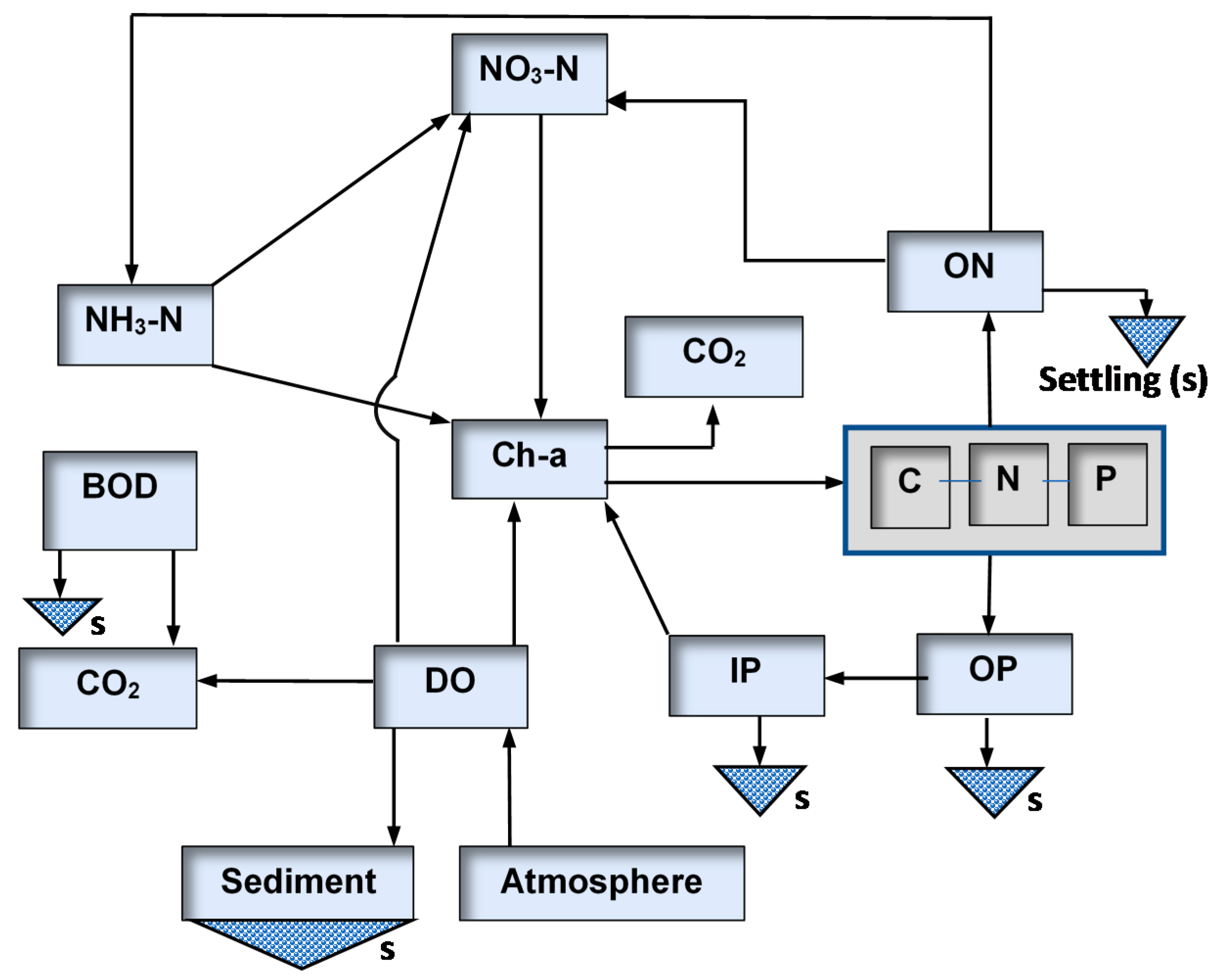
The advanced eutrophication module is the most complicated module, which incorporates different parameters of eutrophication. This module includes many mass-balance equations to calculate the fate, transport, transformations, phytoplankton, as well as BOD, DO, and nitrification dynamics [46,47,48]. Interactions, components, and structure considered in the WASP model are shown in Figure 2. Carbonaceous organic materials in water exert oxygen uptake in the process releasing CO2 as an ingredient for Chlorophyll-a formation. The residual organic particulates then settle to form the sediment composition. The death of plants yields and releases C-N-P constituent matter into the water column. Aquatic plants require basic nutrient constituents of carbon, nitrogen, and phosphorus for energy and tissue development. Their growth and death dynamics can be monitored by the changes of Chlorophyll-a concentration in the water body. Photosynthesis processes involve the oxidation of organic and inorganic forms of the nutrient constituent in water transformed through as dynamic interrelated interactions causing and driven by eutrophication processes. The insoluble Inorganic Phosphate (IP), Organic Phosphates (OP), insoluble Organic Nitrate (ON), and carbonaceous inorganic particles settle through the water column and integrate into the sediment, forming a dynamic benthic-nutrient structure. (represented by triangles). The general equation used for the calculation of any water-quality variable is a mass-balance equation, which could be stated as Equation (1):
In Equation (1), S is the concentration of water-quality variables, U is the average velocity, A is the area of cross-section, x is the distance in 1 dimension (In the direction of flow from loading source), and t is time. Whereas E is the longitudinal dispersion coefficient, SC is the external and internal sinks and sources.
2.4. Model Physical Domain
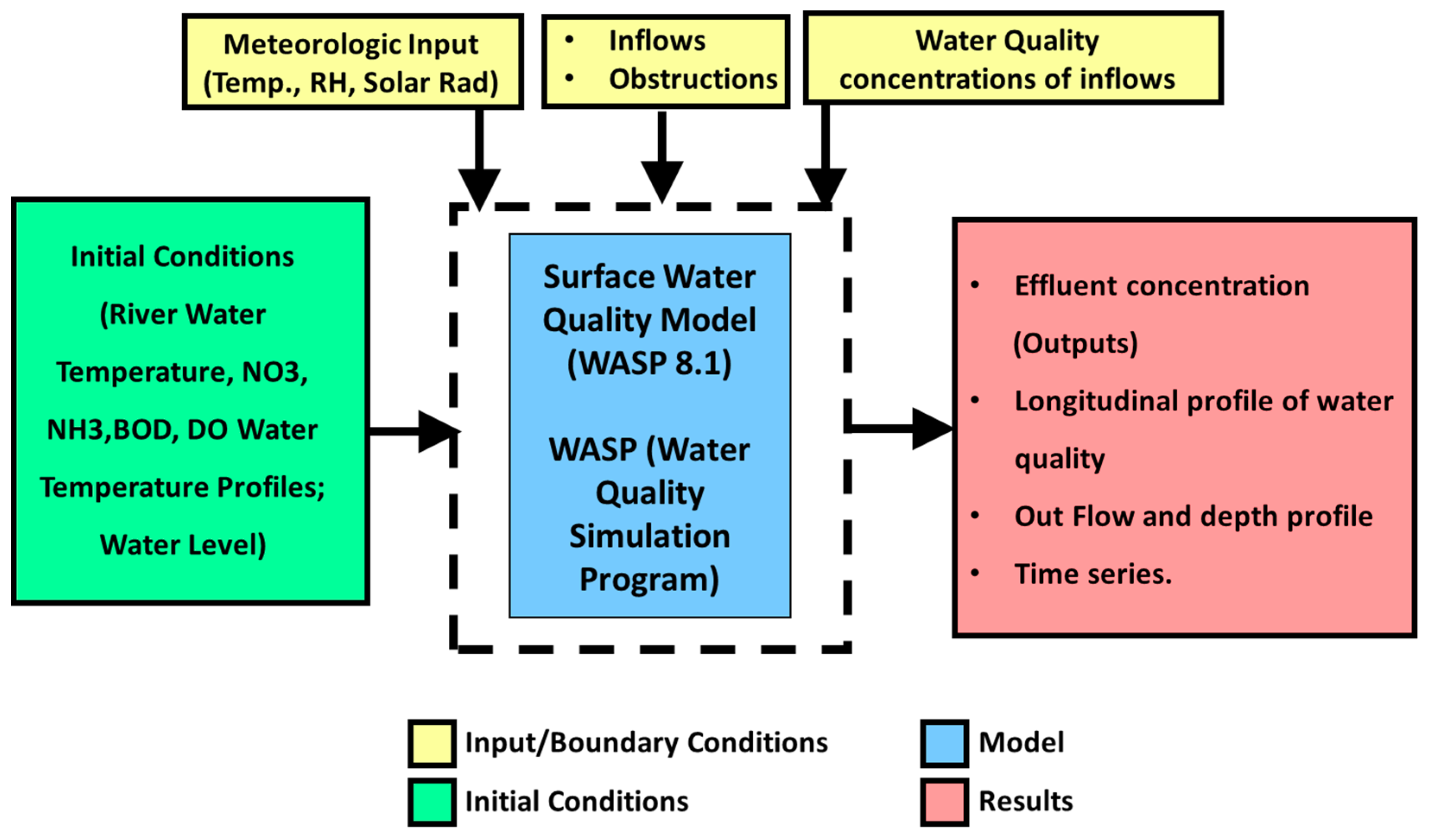
The model physical domain consists of the data sets, system (model state-variable activation), segments (segment definition and initial conditions), environmental parameters, calibration constants, flows (channel geometry and surface waters), boundaries (concentration inputs of activated parameters), out-control, and fluxes of water-quality parameters. The short explanation of the flow of the model is described in Figure 3.
2.4.1. River Discretization
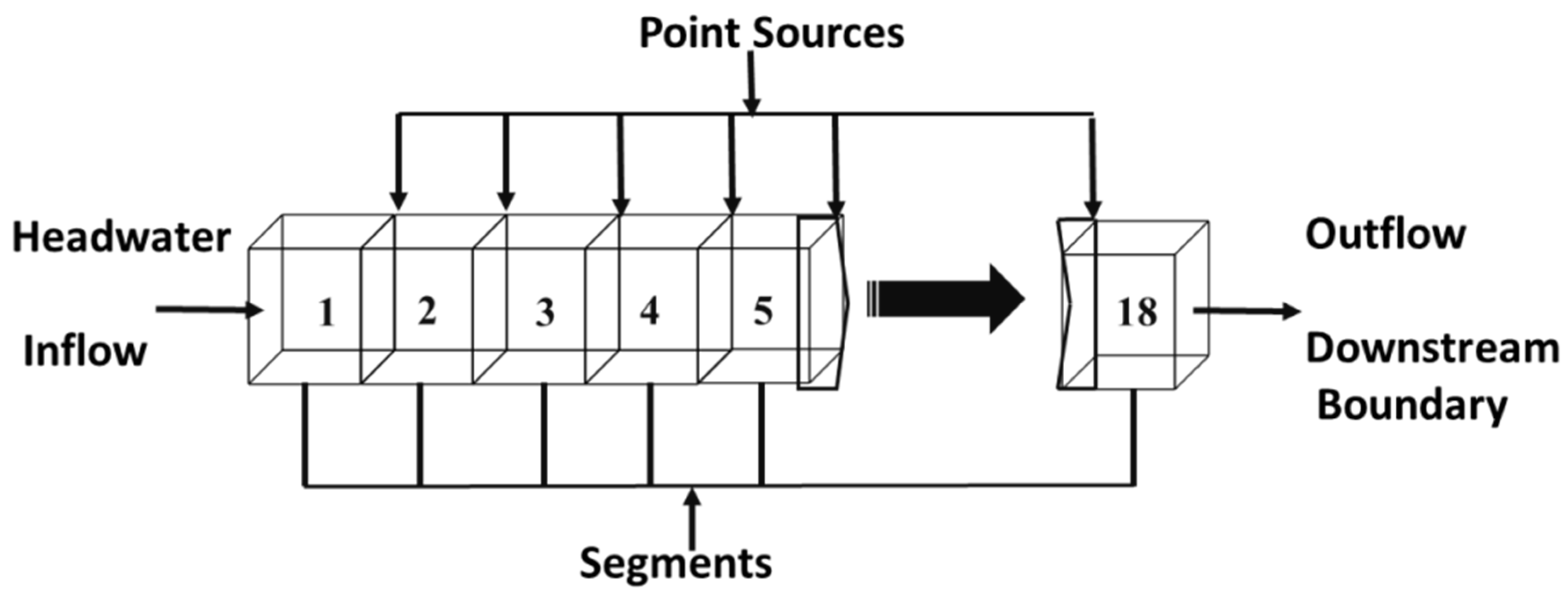
The model setup comprises 18 horizontal segments; each segment is the distance between 2 consecutive point outlets. However, the length of the first segment is the distance between the headwater and the first point-source outlet while the length of the last segment is the distance between the last point-source outlet to the downstream boundary. The upstream location of the first segment is the headwater, and the downstream location of the last segment is the downstream-boundary condition. Figure 4 shows the example of horizontal-flow segmentations used in the WASP model and location of point sources and segments along the section of the Ravi River.
2.4.2. Initial and Boundary Conditions
The water inflows are consisting of the inflow coming from India, inflows from link canals, and inflows from drains. All the inflow data obtained were measured by the WAPDA, PIDA, and WASA to develop the water-inflow files to input in the WASP model. The initial condition describes the initial state of water bodies before running the model. The initial condition is only required when modeling is conducted under time-dependent conditions. Under a steady-state modeling approach, by definition, the initial condition is not important [49]. However, this study used an average of the mainstream observation of the Ravi River at 6 different locations as initial conditions. In our study, based on the availability of measured data of water-quality parameters, we used 6 water quality variables consisting of TDS, NH3-N, NO3-N, BOD, DO, and temperature. All these 6 variables were considered for the initial and boundary conditions. Due to the Indus Basin Treaty between India and Pakistan, the flow of eastern rivers (Ravi, Sutlej, Beas) reduced significantly compared to the western rivers (Indus, Jhelum, Chenab). Therefore, in Pakistan, link canals have been constructed to connect the water flow of western rivers (Indus, Jhelum, Chenab) to eastern rivers (Ravi, Sutlej) to cope with the shortage of water in the region. Link canals also carry the pollution loads of many small drains that come in the passages of these canals. The main source of contamination of the Ravi River is wastewater drains that flow into the Ravi River. These drains carry the industrial and sewage wastewater of urban areas along the sections of the river. Hence, flow masses of drains and link canals are added as point-source tributaries. In addition, meteorological data, including wind speed, solar radiation, rainfall, and air temperature were obtained from the PMD and were used for the construction of boundary conditions.
2.4.3. Input Data and Model Outputs
WASP is capable of simulating pollutant concentrations up to 3 dimensions in steady state and dynamic mode. The current study used steady-state mode for simulation of fate and solute transport in one dimension. The measured water velocities and river geometries were used to calculate the coefficient and exponent of velocities and depth at sampling locations, which could be stated as Equations (2) and (3):
The exponents β, δ and coefficients α, γ were computed using velocities, flow, and mean depth. The water-quality input parameters for model simulation included DO, BOD, TDS, NO3-N, NH3-N, and temperature. The environmental parameters included were meteorological information, such as wind speed, rainfall, relative humidity, and air temperature. The model can simulate multiple water-quality parameters simultaneously such as BOD, DO, DO deficit, Dissolved Organic Carbon (DOC), temperature, NO3-N and NH3-N, NH4+-N, Total Organic Nitrogen (TON), Total Inorganic Nitrogen (TIN), Dissolved Organic Nitrogen (DON), Dissolved Inorganic Nitrogen (DIN), TN, pH, TSS, TDS, phosphorous, and macro-algae compounds. However, the model GUI provides an output-control option and, from this output-control option, we can select the desired water-quality parameters to be simulated and the rest of the parameters neglected by the model. For calibration and validation purposes, the model was manually fitted by tuning the different modeling parameters and reaction constants for 6 water quality variables, i.e., BOD, TDS, DO, NO3-N, NH4-N, and temperature.
2.5. Scenario Development for Pollution-Concentration Control
This study developed a total of 7 scenarios for water-quality management to control pollution concentration (Table 2). The 7 management scenarios as follows were: (1) Headwater increased up to 50% more than the existing flow (23 m3/s). In the past 4 decades, the average annual inflow of the Ravi River has declined 10 times at the entrance point in Pakistan, while in India the average discharge is still 267.5 m3/s (near Mukesar, India) [41,50]. (2) The water in link canals increased up to 50% more than the existing water flow; these canals were constructed with much more capacity than the existing flow. (3) Both flows at the headwater and link canals increased up to 50% more than the existing flow, i.e., scenario (1) plus (2). (4) If water-treatment facilities are installed in the drains carrying municipal and industrial wastewater, with 75% improvement in pollution concentration. (5) Headwater flow increase by 50% plus water treatment of drains, i.e., scenario (1) plus (4). (6) The increase of link-canal flow by 50% plus wastewater treatment of drains, i.e., scenario (2) plus (4). (7) Both headwater and link-canal flow increased by 50% plus application of water-treatment facilities in waste-carrying drains, i.e., scenario (3) plus (4).
The Indus basin river system consists of 6 main rivers, i.e., Indus (the longest), Jhelum, Chenab, Ravi, Sutlej, and Beas. All the rivers originated from India. Due to political issues and the Indus Basin Water Treaty, the water of the Indus basin rivers is divided between India and Pakistan. India has control over eastern rivers, while Pakistan has more access to the water of western rivers. The major rationale behind the 50% increase of flow is that the average annual discharge in the Ravi River near Mukesar, India is about 267.5 m3/s [41]. As the river enters Pakistan, the discharge of the Ravi River is reduced to about 23 m3/s at the upstream of the Marala Ravi Link Canal (headwater/starting point of study). This flow is much less than the “minimum environmental flow” (the minimum quantity of water flow required to sustain freshwater, river ecosystem, human beings, and other species that depend upon a water ecosystem). Usually, it is considered that 15–18% is the minimum environmental flow than that of the actual flow [51,52,53,54].
So, this study proposed that by mutual agreement if Pakistan buy some water from India up to the minimum environmental water flow for the survival of poor water quality and moderate habitat, it would bring positive effects on the health of the Ravi River ecosystem. The 50% increase of water in the Ravi River means 50% more flow than the existing 23 m3/s from upstream, which is around 35 m3/s (minimum environmental flow). As water flow in the western river is much more than eastern rivers in Pakistan, to cope with the shortage of water and conserve the ecosystem, Pakistan had constructed link canals that connected the water of western rivers with eastern rivers. These link canals have been designed with much more capacity than the existing flow. As the surrounding command area of the Ravi River is composed of fertile agriculture land, if the water in link canals increased more than the existing flow, it would not only conserve water quality and habitats but could also bring positive effects on the region’s agriculture economy. However, the main concern is to improve poor water quality and habitat ecosystem; therefore, only the flow increment by link canals is not feasible, because as the Ravi River enters Pakistan the first link canal connects with the Ravi River 50 km downstream of the river. Link canals can improve the river ecosystem after 50 km; therefore, the first 50 km can be improved by increasing the inflow up to the minimum environmental flow of the Ravi River. That’s why the authors have proposed flow augmentation both at link canals and the upstream location. The scenarios proposed in this study have considered the minimum limits and maximum possibilities. Most wastewater treatment plants can reduce the pollution load by up to 75–85%. Therefore, this study provides the scenarios considering the least favorable conditions, i.e., 50% flow, and 75% reduction of pollution loads. However, if flow is increased or very high-efficiency wastewater-treatment facilities are installed, the health of the Ravi River ecosystem will be further improved.
2.6. Model Application and Calibration
The study utilized the WASP 8.1 model for simulating the longitudinal water-quality profile along the course of the selected region of the Ravi River channel. The total length of the selected study river from upstream (M1) to downstream (M6) is around 220 km. The measured data of the 1st event (17–18 April 2018) were used for the model calibration. The inflow and water quality concentration of 14 drains (D1–D14) and 3 link canals (C1–C3) were impeded into the domain of the WASP model as inputs. Meteorological information, including wind speed, radiation, air temperature, humidity, cloud coverage, and rainfall was obtained from the PMD and was used to make the meteorological input files. The water-quality data obtained in the other 2 events were used for validation of the model results. The model was manually fitted by tuning the different modeling parameters and reaction constants for 6 water quality variables, i.e., BOD, TDS, DO, NO3-N, NH4-N, and temperature.
2.7. Model Accuracy Evlauation
The model performance was evaluated by comparing the measured and predicted data. The following 5 statistical estimators were used to evaluate the accuracy of the calibrated and validated results suggested by the previous studies [55,56,57,58,59,60].
The coefficient of determination (R2) measures goodness of fit between observed and predicted data. The value of R2 ranges from 0 to 1. If the value of R2 is close to 1, the model prediction fits well with measured data.
The mean absolute error (MAE) measures the absolute quantitative deviation among observation and predicted results. The MAE formula is given as:
The normalized root mean square error (NRMSE) measures the overall variation among predicted and observed values. As the size of the error decreases, prediction accuracy increases.
The mean absolute percentage error (MAPE), an estimator, measures the percentage deviation among simulated and measure results.
The percentage model bias (PMB) is a measure of the model under/overestimations of the field observations. The lower the PMB, the higher the model prediction accuracy.
Here, O is the observed value measured from the mainstream sampling location, S is the simulated value obtained from the model result for a similar profile location, where field observation was conducted for model calibration and validation, N is the total number of all the measured data, and i is the ith comparison. The mean value of O and S is the average value of the observed data and the simulated model results from the corresponding mainstream observation location, respectively.
3. Results and Discussion
3.1. Model Calibration and Validation
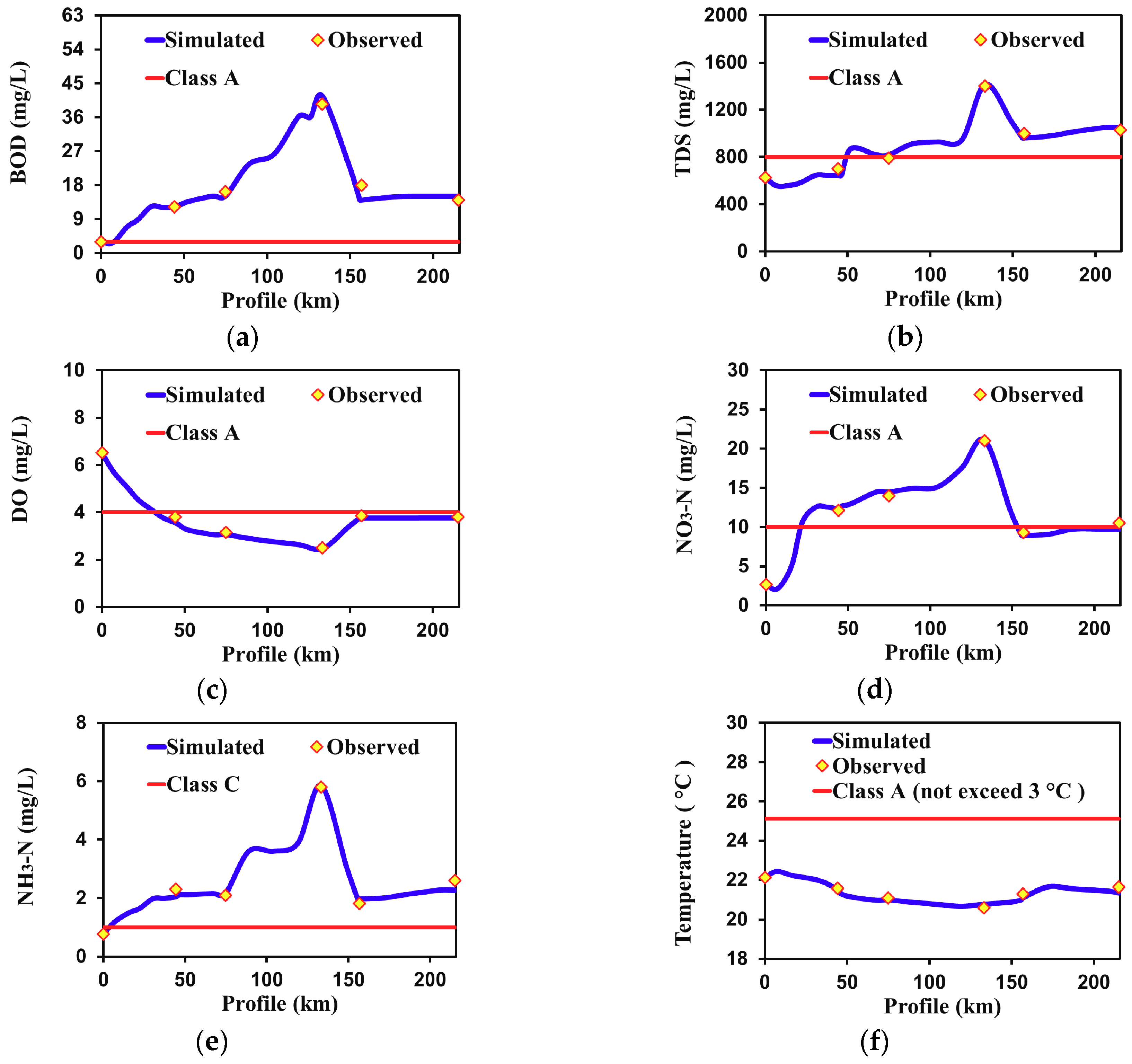
Water-quality data, inflow information, and meteorological data for the first event were used for the model calibration by comparing simulated and measured data; environmental, stoichiometric, and kinetics parameters were manually adjusted to obtain reasonable results (Table 3). Figure 5 and Figure 6 show the calibrated and validated results of TDS, NH3-N, NO3-N, BOD, DO, and temperature of the Ravi River, respectively.
The result shows that the water-quality profile of the Ravi River after the discharge of wastewater-carrying drains is extremely degraded based on the National Water Quality Standard (Table 4) in terms of all studied variables. For example, in the downstream segment of the Hudiara drain, concentrations of TDS, NH3-N, NO3-N, BOD, and DO is 1180 mg/L, 5.85 mg/L, 20.77 mg/L, 37.13 mg/L, and 2.47 mg/L, respectively. The water quality of the Ravi River at upstream, where the water flows from headwater and the Marala Ravi link canal, was much better than the mid- and downstream locations, which are close to urban municipalities and therefore directly affected by wastewater-carrying drains. The oxygen sag was clearly observed between upstream and 125 km; however, after the addition of fresh water inflow from link canals (Upper Chenab canal and Qadrabad Balloki link canal), the DO curve tends to increase.
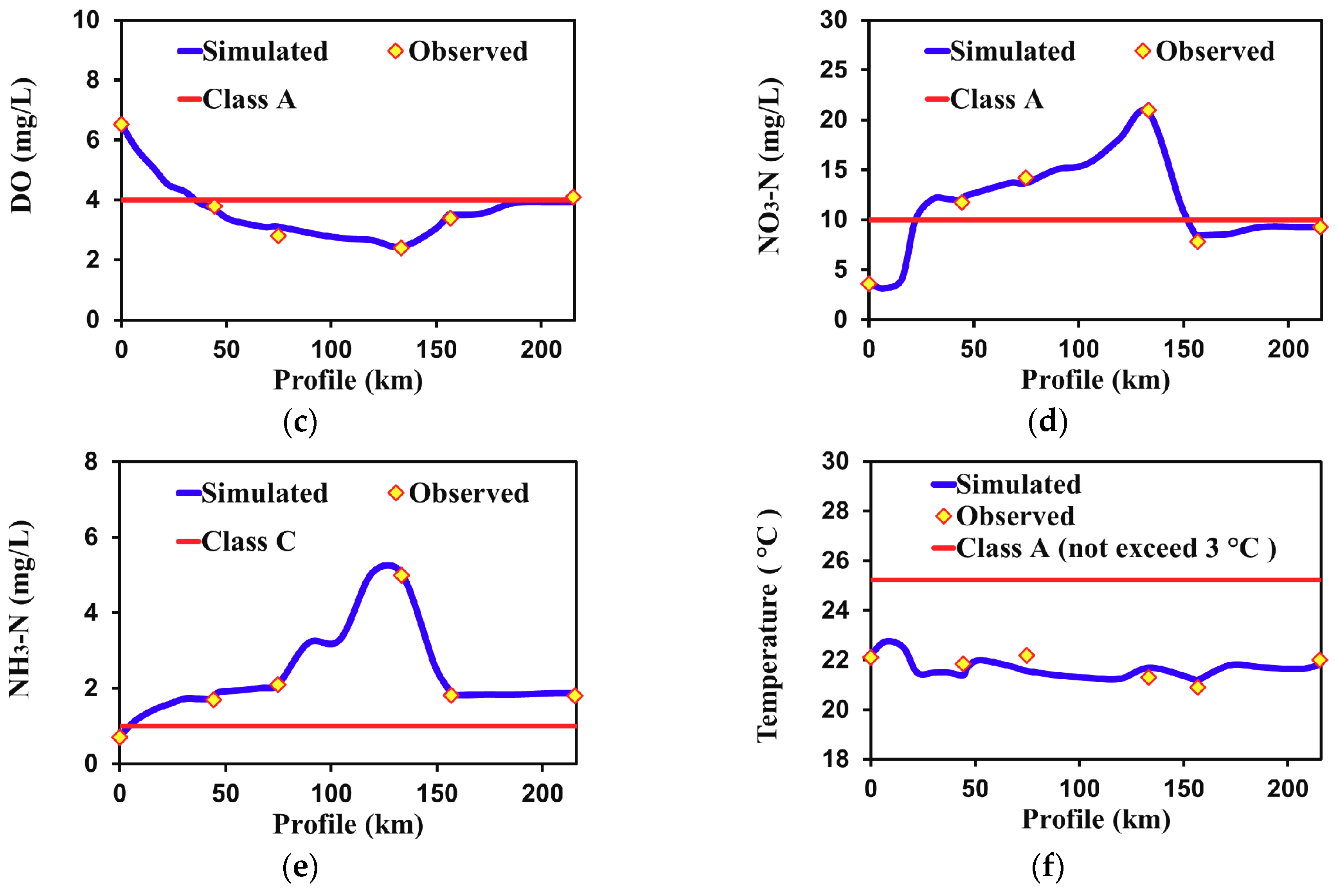
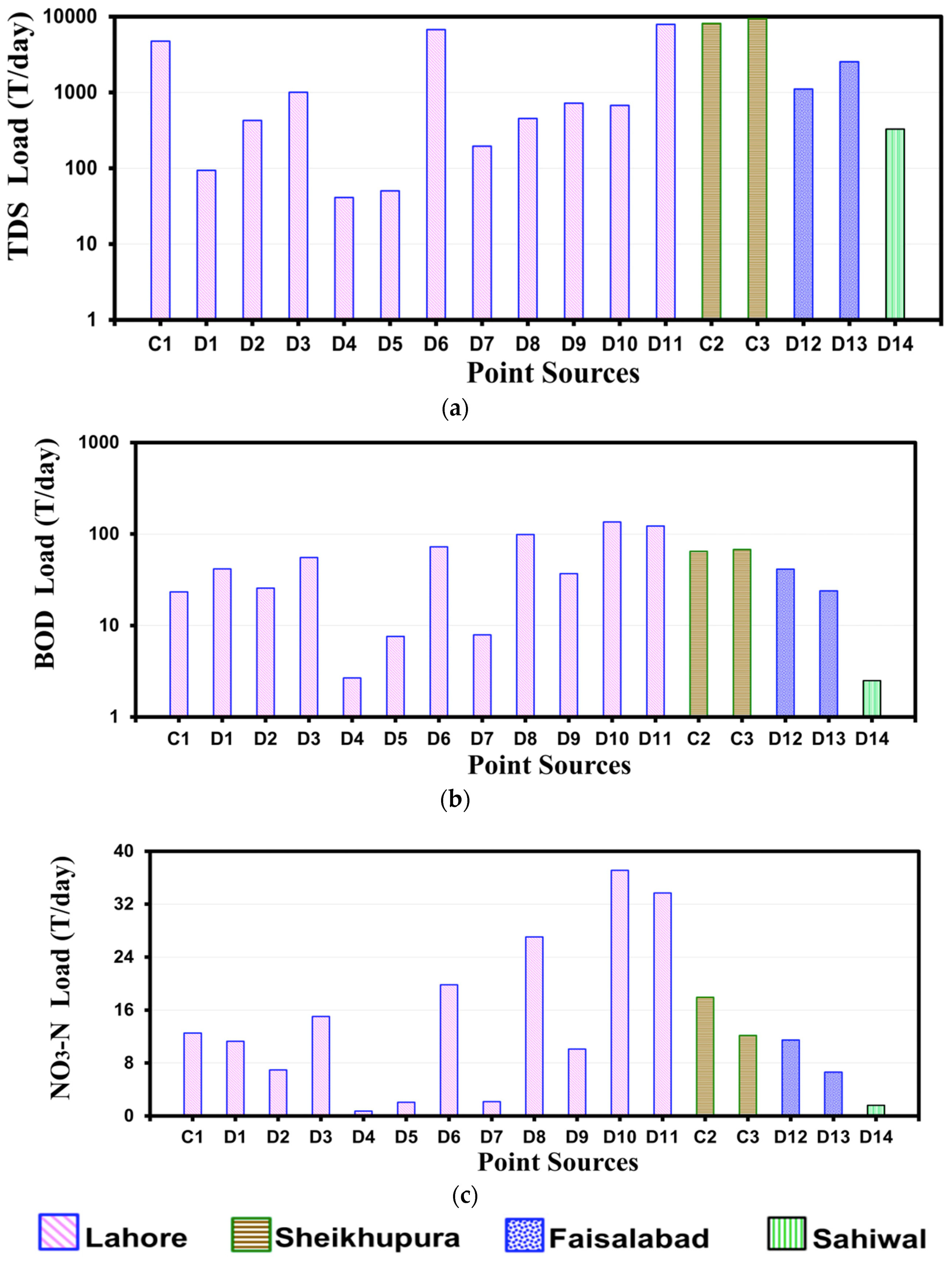
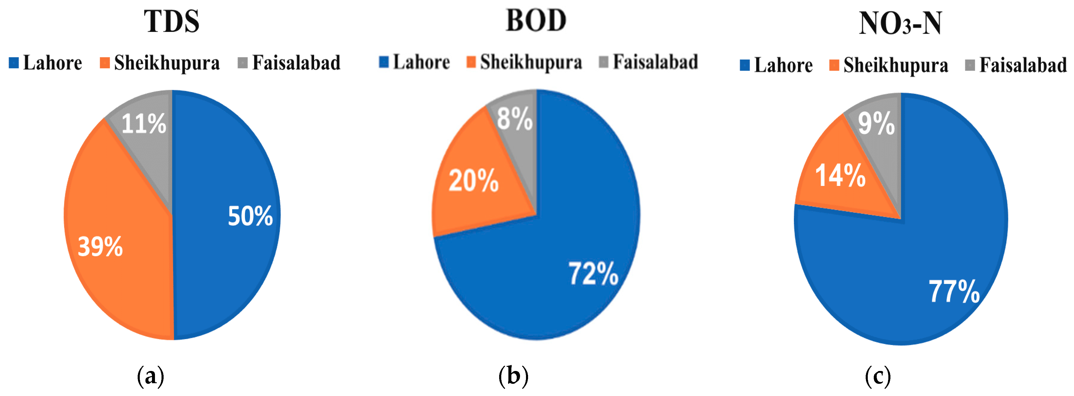
The pollution loads (in tons per day) of all drains discharging into the Ravi River directly or indirectly (via link canals) are shown in Figure 7 along the section of Ravi River. Results reveal that most of the pollution load is discharged into the Ravi River from the municipality of Lahore, which is the most populous city [36] of Punjab, Pakistan. Another reason for the highest share of the pollution load by Lahore is that the Ravi River passes through the center of Lahore and all the major wastewater-carrying drains fall into the Ravi River.
Among all waste-carrying drains, the Farukhabad and Hudaira drains carry significant shares of the pollution load. Farukhabad carries both industrial and sewage waste from the municipality of Sheikhupura Road, Shadra, Baradari Road, G.T. Road, and the suburbs of these vicinities. The Hudiara drain is another of the biggest drains, which carries domestic and industrial waste of township residential areas, township industrial estates, the towns of Johar, Faisal, and WAPDA, and the wastewater of small drains, including the Nishtar Colony drain, Sattokatla drain, and Charrar drain. Overall, the Ravi River receives the highest share of pollution load from Lahore, followed by the Sheikhupura and Faisalabad district municipalities (Figure 8). The share of pollution load from the Sahiwal district via the Sukhrawa drain is 0.25%, which is negligible.
The high value of R2 (close to 1) and lower values of statistical errors, i.e., MAE, NRMSE, MAPE, and PMB indicated that the model fitted well with the measured data, both for calibrated and validated results. Table 5 shows that the model agrees well with the measured data up to some extent. To support decision making and management planning, the calibrated model is further applied with different management strategies (Table 2).
3.2. Strategies to Control Pollution Concentration
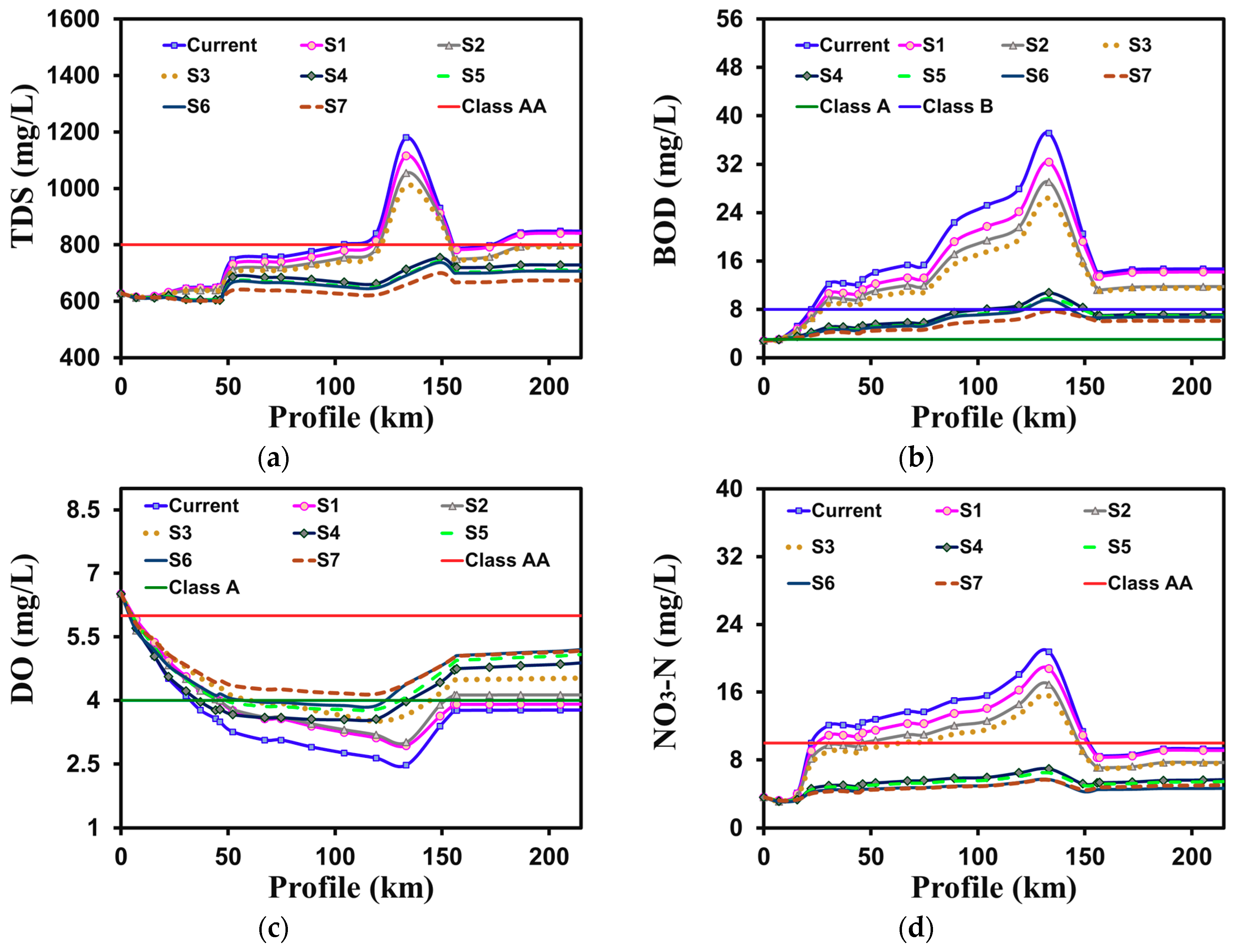
The study evaluated the water-quality concentration along the section of the Ravi River with seven different scenario-based management strategies. The possible water-quality enhancement was assessed based on each management scenario listed in Table 2. Variables like BOD, DO, TDS, and NO3-N are commonly adopted in many countries as water-quality standards. So, they were selected as performance indicators to examine the result of management scenarios (Figure 9). The Ravi River was divided into eighteen segments and each segment has a defined length of induvial point sources. The model simulation was performed for each management scenario, and results of each scenario were compared with the current conditions. After applying all seven management strategies, a significant improvement was found in the longitudinal profile of water quality (Figure 9).
Based on these management scenarios (flow augmentation, water treatment facilities, and local oxygenation) significant water-quality improvement was observed. With the application of these management strategies, TDS and NO3-N levels were improved for public supply water quality I (Class AA) (Figure 9a,d and Table 4), while DO was improved for public supply II (Class A) (Figure 9c). However, maximum BOD simulated was 7.73 mg/L (Class B) with the seventh management scenario (Figure 9b), which is considered reasonable for developing South Asian countries [62].
The potential improvement in the water-quality profile of the most polluted segment from the headwater is shown in Table 6. The increased flowrate affects the water quality through dilution and the introduction of wastewater-treatment plants improves the water quality by providing treated water. Overall, the highest improvement was observed at the most polluted segment of the river, which is located just below the downstream of the Hudiara drain, which has the highest share of pollution load among all waste-carrying drains. The least percentage improvement of TDS concentration was observed in the first scenario and most difference was seen in the seventh scenario. The most significant change in the water-quality profile was observed after the application of wastewater-treatment facilities. Overall, the wastewater-treatment application has more effect than the dilution effect on the concentration of TDS. However, the combined effect of both dilution and wastewater facilities improves the overall health of the river ecosystem. In the case of BOD contradictory to the TDS, a more significant improvement was observed with the application of flow augmentation. This can be attributed to the fact that headwater and link-canal concentration of BOD was much smaller than the downstream of the river. Therefore, before the introduction of wastewater-treatment plants, the percentage change in the concentration with flow augmentation both from link canals and headwater was observed as 28.99%. However, with the introduction of wastewater-treatment facilities, this percentage change inclined to 71.03%, which can be concluded that, similarly to the TDS, the wastewater-treatment plant has more influence than the dilution effect. Water having good quality holds more oxygen than water having poor quality, which contains less dissolved oxygen.
Similar to the previous two cases, the increasing improvement trend of dissolved oxygen concentration was observed. However, contradictory to the first two cases, the wastewater-treatment facility does not increase the dissolved oxygen. To this end, the local oxygenation should be considered, which is the inclusion of “aeration blowers” in the wastewater-treatment facilities or construction of weirs in the section of wastewater-carrying drains [63]. Similar to the previous three cases, the decreasing trend in the mean concentration of NO3-N was observed from scenario one to scenario seven.
From this assessment, it was found that the large drains are more responsible for the contamination of the river, such as the Hudiara drain. Therefore, a Large-scale Biological Nutrient Removal (BNR) system [64,65,66] should be installed to improve drain-water quality. However, in case of small drains, simple physical and chemical unit operations would be enough for water treatment [4]. Consequently, dissolved air floatation [67,68,69] could also reduce up to 80% of suspended solids and phosphorous, while anammox biocathode could remove up to 90% ammonium [70]. Furthermore, a least-operating-cost electrocoagulation (EC) using aluminum electrodes can remove TDS and BOD up to 70–80% [71]. The study also suggests that if inflow from neighboring drains is converted and collected at one point, treatment cost could be reduced significantly.
4. Conclusions
The WASP model in steady-state mode was calibrated and validated using the data for the year 2018. The model shows quite good agreement against the field data, with some exceptions. Furthermore, this study applied to a total of seven management strategies to control the pollution concentration of the Ravi River. The study found that the water quality of the Ravi River would improve most significantly if inflow from link canals and headwater was increased and treatment facilities were designed for sewage and industrial waste-carrying drains (Scenario 7).
When fresh-water inflow was assumed to be increased by 50% and the treatment efficiency of a wastewater-treatment plant, along with local oxygenation, was assumed to be 75%, the Ravi River water quality could be classified in Class B in case of BOD, Class A in case of DO, Class AA in case of NO3-N and TDS with comparison to the local water-quality standards. The study shows that wastewater-treatment facilities along with local oxygenation are effective to control the pollution concentration of waste-carrying drains. The combination of flow augmentation both from headwater and link canals and wastewater-treatment facilities along with local oxygenation is suitable to keep the water quality of the Ravi River within acceptable limits. These management scenarios will be helpful in policy making for urban planning. Sustainable water-quality management should be incorporated by a combination of various strategies, including minimum environmental inflow regulation, reduction in wastewater generation, and wastewater treatment.
Furthermore, it is recommended that a long-term and continued monitoring program should be established to forecast the water quality of the river. Data from the monitoring program could be used for updating the model calibration and validation processes described in this paper. Moreover, the introduction of a forecasting system using automatic wireless-sensor networks for water-quality monitoring also enables the administration to keep the concentration of the contaminants to the desirable level by tracking the real-time changes of the water quality in order to anticipate any changes caused by environmental or manmade activities.
Supplementary Materials
The following are available online at https://www.mdpi.com/2073-4441/10/8/1068/s1, Table S1–S3: Water quality measurement data collected along the Ravi River (three different sets of survey data).
Author Contributions
M.M.I., M.S., P.A. and J.L.L. designed the study; J.L.L. guided and supervised the study; M.M.I. and M.S. analyzed and simulated the data; and M.M.I. wrote the article.
Funding
This research work was supported by the Graduate School of Water Resources, Sungkyunkwan University, and the APC was funded by the Coastal and Environmental Laboratory, Sungkyunkwan University. The first and second author were supported through a scholarship program ((HRDI-UESTP) by the Higher Education Commission (HEC), Pakistan.
Acknowledgments
The authors are grateful to S.H., Department of Irrigation and Drainage, University of Agriculture, Faisalabad, for helping in water quality sampling. We also want to acknowledge A.A.L., Department of Water Resources, Sungkyunkwan University, for helping in the editing and proofreading of the manuscript.
Conflicts of Interest
The authors declare no conflict of interest.
References
- Bekele, E.; Page, D.; Vanderzalm, J.; Kaksonen, A.; Gonzalez, D. Water recycling via aquifers for sustainable urban water quality management: Current status, challenges and opportunities. Water 2018, 10, 457. [Google Scholar] [CrossRef]
- Galvis, A.; Van der Steen, P.; Gijzen, H. Validation of the three-step strategic approach for improving urban water management and water resource quality improvement. Water 2018, 10, 188. [Google Scholar] [CrossRef]
- Almaarofi, H.; Etemad-Shahidi, A.; Stewart, R.A. Strategic evaluation tool for surface water quality management remedies in drinking water catchments. Water 2017, 9, 738. [Google Scholar] [CrossRef]
- Lee, I.; Hwang, H.; Lee, J.; Yu, N.; Yun, J.; Kim, H. Modelling approach to evaluation of environmental impacts on river water quality: A case study with Galing River, Kuantan, Pahang, Malaysia. Ecol. Model. 2017, 353, 167–173. [Google Scholar] [CrossRef]
- Jalilov, S.; Kefi, M.; Kumar, P. Sustainable urban water management: Application for integrated assessment in Southeast Asia. Sustainability 2018, 10, 122. [Google Scholar] [CrossRef]
- UN Water. UN-Water Annual Report 2008. Available online: http://www.unwater.org/downloads/annualreport2008.pdf (accessed on 22 May 2018).
- Mishra, B.K.; Regmi, R.K.; Masago, Y.; Fukushi, K.; Kumar, P.; Saraswat, C. Assessment of Bagmati river pollution in Kathmandu Valley: Scenario-based modelling and analysis for sustainable urban development. Sustain. Water Qual. Ecol. 2017, 9, 67–77. [Google Scholar] [CrossRef]
- Wang, Z.; Zou, R.; Zhu, X.; He, B.; Yuan, G.; Zhao, L.; Liu, Y. Predicting lake water quality responses to load reduction: A three-dimensional modelling approach for total maximum daily load. Int. J. Environ. Sci. Technol. 2014, 11, 423–436. [Google Scholar] [CrossRef]
- Rashidi, H.; Ghaffarianhoseini, A.; Ghaffarianhoseini, A.; Nik Sulaiman, N.M.; Tookey, J.; Hashim, N.A. Application of wastewater treatment in sustainable design of green built environments: A review. Renew. Sustain. Energy Rev. 2015, 49, 845–856. [Google Scholar] [CrossRef]
- Srinivas, R.; Singh, A.P. An integrated fuzzy-based advanced eutrophication simulation model to develop the best management scenarios for a river basin. Environ. Sci. Pollut. Res. 2018, 25, 9012–9039. [Google Scholar] [CrossRef] [PubMed]
- Li, K.; He, J.; Li, J.; Guo, Q.; Liang, S.; Li, Y.; Wang, X. Linking water quality with the total pollutant load control management for nitrogen in Jiaozhou Bay, China. Ecol. Indic. 2018, 85, 57–66. [Google Scholar] [CrossRef]
- Bieroza, M.Z.; Heathwaite, A.L.; Bechmann, M.; Kyllmar, K.; Jordan, P. The concentration-discharge slope as a tool for water quality management. Sci. Total Environ. 2018, 630, 738–749. [Google Scholar] [CrossRef] [PubMed]
- Slaughter, A.R.; Hughes, D.A.; Retief, D.C.H.; Mantel, S.K. A management-oriented water quality model for data scarce catchments. Environ. Model. Softw. 2017, 97, 93–111. [Google Scholar] [CrossRef]
- Chen, Y.; Shuai, J.; Zhang, Z.; Shi, P.; Tao, F. Simulating the impact of watershed management for surface water quality protection: A case study on reducing inorganic nitrogen load at a watershed scale. Ecol. Eng. 2014, 62, 61–70. [Google Scholar] [CrossRef]
- Gao, L.; Li, D. A review of hydrological/water-quality models. Front. Agric. Sci. Eng. 2014, 1, 267. [Google Scholar] [CrossRef] [Green Version]
- Nguyen, T.T.; Keupers, I.; Willems, P. Conceptual river water quality model with flexible model structure. Environ. Model. Softw. 2018, 104, 102–117. [Google Scholar] [CrossRef]
- Cox, B.A. A review of currently available in-stream water-quality models and their applicability for simulating dissolved oxygen in lowland rivers. Sci. Total Environ. 2003, 314, 335–377. [Google Scholar] [CrossRef]
- Tsakiris, G.; Alexakis, D. Water quality models: An overview. Eur. Water 2012, 37, 33–46. [Google Scholar]
- Wang, Q.; Li, S.; Jia, P.; Qi, C.; Ding, F. A review of surface water quality models. Sci. World J. 2013, 2013. [Google Scholar] [CrossRef] [PubMed]
- Morley, N.J. Anthropogenic effects of reservoir construction on the parasite fauna of aquatic wildlife. Ecohealth 2007, 4, 374–383. [Google Scholar] [CrossRef]
- Wang, Y.; Hua, Z.; Wang, L. Parameter estimation of water quality models using an improved multi-objective particle swarm optimization. Water 2018, 10, 32. [Google Scholar] [CrossRef]
- Yan, Z.; Wang, Y.; Wu, D.; Xia, B. Exploration of an urban lake management model to simulate chlorine interference based on the ecological relationships among aquatic species. Sci. Rep. 2018, 8, 8325. [Google Scholar] [CrossRef] [PubMed]
- Zhu, S.; Zhang, Z.; Liu, X. Enhanced two dimensional hydrodynamic and water quality models (CE-QUAL-W2) for simulating mercury transport and cycling in water bodies. Water 2017, 9, 643. [Google Scholar] [CrossRef]
- Kannel, P.R.; Kanel, S.R.; Lee, S.; Lee, Y.S.; Gan, T.Y. A review of public domain water quality models for simulating dissolved oxygen in rivers and streams. Environ. Model. Assess. 2011, 16, 183–204. [Google Scholar] [CrossRef]
- Ambrose, R.B.; Wool, T.A. WASP8 Stream Transport—Model Theory and User’s Guide Supplement to Water Quality Analysis Simulation Program (WASP) User Documentation; United Sates Environmental Protection Agency: Athens, GA, USA, 2017.
- Ambrose, R.B.; Wool, T.A.; Martin, J.L. The Water Quality Analysis Simulation Program, WASP5 Part A: Development Protection Agency; United States Environmental Protection Agency: Athens, GA, USA, 1993.
- Akomeah, E.; Chun, K.P.; Lindenschmidt, K.E. Dynamic water quality modelling and uncertainty analysis of phytoplankton and nutrient cycles for the upper South Saskatchewan River. Environ. Sci. Pollut. Res. 2015, 22, 18239–18251. [Google Scholar] [CrossRef] [PubMed]
- Yang, C.P.; Lung, W.S.; Kuo, J.T.; Lai, J.S.; Wang, Y.M.; Hsu, C.H. Using an integrated model to track the fate and transport of suspended solids and heavy metals in the tidal wetlands. Int. J. Sediment Res. 2012, 27, 201–212. [Google Scholar] [CrossRef]
- Yang, C.; Kuo, J.; Lung, W.; Lai, J.; Wu, J. Water quality and ecosystem modelling of tidal wetlands. J. Environ. Eng. 2007, 133, 711–721. [Google Scholar] [CrossRef]
- Yao, H.; Qian, X.; Yin, H.; Gao, H.; Wang, Y. Regional risk assessment for point source pollution based on a water quality model of the taipu river, China. Risk Anal. 2015, 35, 265–277. [Google Scholar] [CrossRef] [PubMed]
- Wang, X.; Jia, J.; Su, T.; Zhao, Z.; Xu, J.; Wang, L. A fusion water quality soft-sensing method based on WASP model and its application in water eutrophication evaluation. J. Chem. 2018, 2018. [Google Scholar] [CrossRef]
- Tang, P.; Huang, Y.; Kuo, W.; Chen, S. Variations of model performance between QUAL2K and WASP on a river with high ammonia and organic matters. Desalin. Water Treat. 2014, 52, 1193–1201. [Google Scholar] [CrossRef]
- Lei, K.; Zhou, G.; Guo, F.; Khu, S.T.; Mao, G.; Peng, J.; Liu, Q. Simulation–optimization method based on rationality evaluation for waste load allocation in Daliao river. Environ. Earth Sci. 2015, 73, 5193–5209. [Google Scholar] [CrossRef]
- Pakistan Bureau of Statistics. Provisional Summary Results of 6th Population and Housing Census 2017. Islamabad. Available online: http://www.pbscensus.gov.pk/ (accessed on 24 May 2018).
- Punjab Bureau of Statistics. Punjab Development Statistics 2017. Lahore. Available online: http://www.bos.gop.pk/publicationreports (accessed on 24 May 2018).
- Rana, I.A.; Bhatti, S.S. Lahore, Pakistan—Urbanization challenges and opportunities. Cities 2018, 72, 348–355. [Google Scholar] [CrossRef]
- Syed, J.H.; Malik, R.N.; Li, J.; Chaemfa, C.; Zhang, G.; Jones, K.C. Status, distribution and ecological risk of organochlorines (OCs) in the surface sediments from the Ravi River, Pakistan. Sci. Total Environ. 2014, 472, 204–211. [Google Scholar] [CrossRef] [PubMed]
- Bilal, C.Q.; Khan, M.S.; Avais, M.; Ijaz, M.; Khan, J.A. Prevalence and chemotherapy of Balantidium coli in cattle in the River Ravi region, Lahore (Pakistan). Vet. Parasitol. 2009, 163, 15–17. [Google Scholar] [CrossRef] [PubMed]
- Baqar, M.; Sadef, Y.; Ahmad, S.R.; Mahmood, A.; Li, J.; Zhang, G. Organochlorine pesticides across the tributaries of River Ravi, Pakistan: Human health risk assessment through dermal exposure, ecological risks, source fingerprints and spatio-temporal distribution. Sci. Total Environ. 2018, 618, 291–305. [Google Scholar] [CrossRef] [PubMed]
- Pakistan Water Gateway. Ravi River Key Facts. 2017. Available online: http://www.waterinfo.net.pk/ (accessed on 18 July 2018).
- Gauging Station Data Summary ORNL; DAAC. Ravi Ravi discharge at Mukesar. 2016. Available online: https://daac.ornl.gov/ (accessed on 24 May 2018).
- JICA (Japan International Cooperation Agency). The Preparatory Study on Lahore Water Supply, Sewerage and Drainage Improvement Project in Islamic Republic of Pakistan, Interim Report, WASA-LDA, Lahore. 2009. Available online: http://open_jicareport.jica.go.jp/ (accessed on 18 July 2018).
- Mahfooz, Y.; Yasar, A.; Bari Tabinda, A.; Sohail, M.T.; Siddiqua, A.; Mahmood, S. Quantification of the River Ravi pollution load and oxidation pond treatment to improve the drain water quality. Desalin. Water Treat. 2017, 85, 132–137. [Google Scholar] [CrossRef]
- Haider, H.; Ali, W. Evaluation of water quality management alternatives to control dissolved oxygen and un-ionized ammonia for Ravi River in Pakistan. Environ. Model. Assess. 2013, 18, 451–469. [Google Scholar] [CrossRef]
- Environment Protection Department. Environmental Monitoring of River Ravi EPA Laboratory December, 2009. 2010. Available online: https://www.epd.punjab.gov.pk/Reports (accessed on 16 May 2018).
- Franceschini, S.; Tsai, C.W. Assessment of uncertainty sources in water quality modelling in the Niagara River. Adv. Water Resour. 2010, 33, 493–503. [Google Scholar] [CrossRef]
- Tufford, D.L.; McKellar, H.N. Spatial and temporal hydrodynamic and water quality Modelling analysis of a large reservoir on the South Carolina (USA) coastal plain. Ecol. Model. 1999, 114, 137–173. [Google Scholar] [CrossRef]
- Vuksanovic, V.; De Smedt, F.; Van Meerbeeck, S. Transport of polychlorinated biphenyls (PCB) in the Scheldt Estuary simulated with the water quality model WASP. J. Hydrol. 1996, 174, 1–18. [Google Scholar] [CrossRef]
- Ji, Z.G. Hydrodynamics and Water Quality Modeling Rivers, Lakes, and Estuaries; John Wiley and Sons, Inc.: Hoboken, NJ, USA, 2009; ISBN 9780470135433. [Google Scholar]
- Wescoat, J.L.; Siddiqi, A.; Muhammad, A. Socio-hydrology of channel flows in complex river basins: Rivers, canals, and distributaries in Punjab, Pakistan. Water Resour. Res. 2018, 54, 464–479. [Google Scholar] [CrossRef]
- Acreman, M.C.; Dunbar, M.J. Defining environmental river flow requirements—A review. Hydrol. Earth Syst. Sci. 2004, 8, 861–876. [Google Scholar] [CrossRef]
- Aguilar, C.; Polo, M.J. Assessing minimum environmental flows in nonpermanent rivers: The choice of thresholds. Environ. Model. Softw. 2016, 79, 120–134. [Google Scholar] [CrossRef]
- Kiwango, H.; Njau, K.N.; Wolanski, E. The need to enforce minimum environmental flow requirements in Tanzania to preserve estuaries: Case study of mangrove-fringed Wami River estuary. Ecohydrol. Hydrobiol. 2015, 15, 171–181. [Google Scholar] [CrossRef]
- Nikghalb, S.; Shokoohi, A.; Singh, V.P.; Yu, R. Ecological Regime versus minimum environmental flow: Comparison of results for a River in a Semi Mediterranean Region. Water Resour. Manag. 2016, 30, 4969–4984. [Google Scholar] [CrossRef]
- Allen, J.I.; Holt, J.T.; Blackford, J.; Proctor, R. Error quantification of a high-resolution coupled hydrodynamic-ecosystem coastal-ocean model: Part 2. Chlorophyll-a, nutrients and SPM. J. Mar. Syst. 2007, 68, 381–404. [Google Scholar] [CrossRef]
- Bae, S.; Seo, D. Analysis and modelling of algal blooms in the Nakdong River, Korea. Ecol. Model. 2018, 372, 53–63. [Google Scholar] [CrossRef]
- Moriasi, D.N.; Arnold, J.G.; Van Liew, M.W.; Bingner, R.L.; Harmel, R.D.; Veith, T.L. Model evaluation guidelines for systematic quantification of accuracy in watershed simulations. Trans. ASABE 2007, 50, 885–900. [Google Scholar] [CrossRef]
- Lewis, K.; Allen, J.I.; Richardson, A.J.; Holt J, T. Error quantification of a high-resolution coupled hydrodynamic ecosystem coastal ocean model: Part 3. Validation with CPR data. J. Mar. Syst. 2006, 63, 209–244. [Google Scholar] [CrossRef]
- Nash, J.E.; Sutcliffe, J.V. River flow forecasting through conceptual models part I—A discussion of principles. J. Hydrol. 1970, 10, 282–290. [Google Scholar] [CrossRef]
- Ostojski, M.S.; Gebala, J.; Orlińska-Woźniak, P.; Wilk, P. Implementation of robust statistics in the calibration, verification and validation step of model evaluation to better reflect processes concerning total phosphorus load occurring in the catchment. Ecol. Model. 2016, 332, 83–93. [Google Scholar] [CrossRef]
- Ministry of Climate Change. National surface water quality guidelines for Pakistan. 2007. Available online: http://www.mocc.gov.pk (accessed on 25 April 2018).
- Kannel, P.R.; Lee, S.; Lee, Y.S.; Kanel, S.R.; Pelletier, G.J.; Kim, H. Application of automated QUAL2Kw for water quality Modelling and management in the Bagmati River, Nepal. Ecol. Model. 2007, 202, 503–517. [Google Scholar] [CrossRef]
- Campolo, M.; Andreussi, P.; Soldati, A. Water quality control in the river Arno. Water Res. 2002, 36, 2673–2680. [Google Scholar] [CrossRef]
- Lakshminarasimman, N.; Quiñones, O.; Vanderford, B.J.; Campo-Moreno, P.; Dickenson, E.V.; McAvoy, D.C. Biotransformation and sorption of trace organic compounds in biological nutrient removal treatment systems. Sci. Total Environ. 2018, 640, 62–72. [Google Scholar] [CrossRef] [PubMed]
- Ogunlaja, O.O.; Parker, W.J. Assessment of the removal of estrogenicity in biological nutrient removal wastewater treatment processes. Sci. Total Environ. 2015, 514, 202–210. [Google Scholar] [CrossRef] [PubMed]
- Estrada-Arriaga, E.B.; Cortés-Muñoz, J.E.; González-Herrera, A.; Calderón-Mólgora, C.G.; de Lourdes Rivera-Huerta, M.; Ramírez-Camperos, E.; Montellano-Palacios, L.; Gelover-Santiago, S.L.; Pérez-Castrejón, S.; Cardoso-Vigueros, L.; et al. Assessment of full-scale biological nutrient removal systems upgraded with physico-chemical processes for the removal of emerging pollutants present in wastewaters from Mexico. Sci. Total Environ. 2016, 571, 1172–1182. [Google Scholar] [CrossRef] [PubMed]
- Dos Santos Pereira, M.; Borges, A.C.; Heleno, F.F.; Squillace, L.F.A.; Faroni, L.R.D. Treatment of synthetic milk industry wastewater using batch dissolved air flotation. J. Clean. Prod. 2018, 189, 729–737. [Google Scholar] [CrossRef]
- Fonseca, R.R.; Thompson, J.P.; Franco, I.C.; da Silva, F.V. Automation and Control of a Dissolved Air Flotation Pilot Plant. IFAC-Pap. Online 2017, 50, 3911–3916. [Google Scholar] [CrossRef]
- Rodrigues, J.P.; Béttega, R. Evaluation of multiphase CFD models for Dissolved Air Flotation (DAF) process. Coll. Surf. Physicochem. Eng. Asp. 2018, 539, 116–123. [Google Scholar] [CrossRef]
- Kokabian, B.; Gude, V.G.; Smith, R.; Brooks, J.P. Evaluation of anammox biocathode in microbial desalination and wastewater treatment. Chem. Eng. J. 2018, 342, 410–419. [Google Scholar] [CrossRef]
- Khandegar, V.; Acharya, S.; Jain, A.K. Data on treatment of sewage wastewater by electrocoagulation using punched aluminum electrode and characterization of generated sludge. Data Br. 2018, 18, 1229–1238. [Google Scholar] [CrossRef] [PubMed]
Figure 1.
Location of study area and sampling points along the Ravi River in Punjab Province, Pakistan.
Figure 1.
Location of study area and sampling points along the Ravi River in Punjab Province, Pakistan.

Figure 2.
Water Quality Simulation Program (WASP) 8.1 graphical illustration of dynamic water-quality parameters: Ammonia as nitrogen (NH3-N), nitrate as nitrogen (NO3-N), Inorganic Phosphorus (IP), Chlorophyll-a (Ch-a), Oxygen Dissolved (DO), Biological Oxygen Demand (BOD), Organic Phosphorus (OP), and Organic Nitrogen (ON).

Figure 3.
Description of model application approach.

Figure 4.
Horizontal segmentations used in the WASP model for the development of the river profile.

Figure 5.
Model calibration of water qualities along the Ravi River for data on 17–18 April 2018: (a) BOD, (b) TDS, (c) DO, (d) NO3-N, (e) NH3-N, and (f) temperature.
Figure 5.
Model calibration of water qualities along the Ravi River for data on 17–18 April 2018: (a) BOD, (b) TDS, (c) DO, (d) NO3-N, (e) NH3-N, and (f) temperature.

Figure 6.
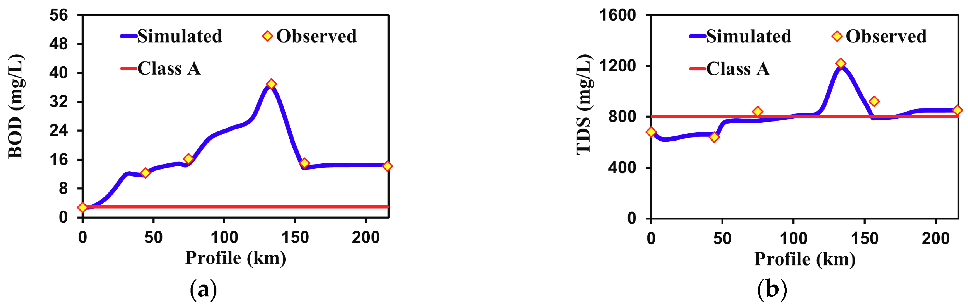
Model validation of water qualities along the Ravi River for data on 17–18 May, 2018 (a) BOD, (b) TDS, (c) DO, (d) NO3-N, (e) NH3-N, and (f) temperature.
Figure 6.
Model validation of water qualities along the Ravi River for data on 17–18 May, 2018 (a) BOD, (b) TDS, (c) DO, (d) NO3-N, (e) NH3-N, and (f) temperature.


Figure 7.
Pollution load contributions of water-quality variables via various link canals and drains along the Ravi River: (a) TDS, (b) BOD, and (c) NO3-N.
Figure 7.
Pollution load contributions of water-quality variables via various link canals and drains along the Ravi River: (a) TDS, (b) BOD, and (c) NO3-N.

Figure 8.
District wise pollution load share of water-quality variables: (a) TDS, (b) BOD, and (c) NO3-N along the Ravi River.
Figure 8.
District wise pollution load share of water-quality variables: (a) TDS, (b) BOD, and (c) NO3-N along the Ravi River.

Figure 9.
Comparison of scenario-based water-quality management results with current conditions along the Ravi River. (a) TDS, (b) BOD, (c) DO, and (d) NO3-N.
Figure 9.
Comparison of scenario-based water-quality management results with current conditions along the Ravi River. (a) TDS, (b) BOD, (c) DO, and (d) NO3-N.


Table 1.
Water-quality sampling location in the Ravi River, drains, and link canals.
| Type | Stations Name | km | Locations |
|---|---|---|---|
| Main River | Miroo Wal (M1) | 0.00 | Meroo Wal, Ravi River before confluence with M.R. Link Canal |
| Railway Bridge (M2) | 44.27 | Upstream of Forest Colony Pumping Station, Railway Bridge | |
| Sughyan Bridge (M3) | 74.84 | Downstream of Bhuda Ravi Drain, Sughyan Bridge | |
| Darbar Bridge (M4) | 133.78 | Downstream of Hudaira Drain, Darbar Syed Imam Ali | |
| Karianwala (M5) | 156.81 | Downstream of Qadrabad Balloki Link Canal, Karianwala | |
| Moza Malayka (M6) | 215.21 | Downstream of Sukhwara Drian, Moza Malayka | |
| Drains | Mehmood Booti Drain (D1) | 15.60 | M.B.D. before confluence with River, near Ring Road |
| Sukh Naher Drain (D2) | 22.13 | S.N.D. before confluence with Ravi River, near Bund Road | |
| Shad Bagh Drain (D3) | 30.30 | S.B.D. before confluence with Ravi River, near Ravi Interchange | |
| Shahdara Town Pumping Station (D4) | 37.08 | S.T.P.S. before confluence with Ravi River, near Shahdara Town Lahore | |
| Forest Colony Pumping Station (D5) | 46.27 | F.C.P.S. before confluence with River Ravi, near Old Bridge Ravi River Lahore | |
| Farukhabad Drain (D6) | 52.12 | Farukhabad Drain before confluence with Ravi river Lahore | |
| Budha Ravi Drain (D7) | 67.20 | B. R. D. before confluence with Ravi River near Munshi Hospital | |
| Main Outfall Drain (D8) | 89.00 | M.O.F.D. before confluence with Ravi River, near Sughyan Lahore | |
| Gulshan-E-Ravi Drain (D9) | 104.21 | G.E.R.D before confluence with Ravi River, near Sanda Bhatiyan | |
| Babu Sabu Drain (D10) | 119.21 | B.S.D. before confluence with Ravi River, near Babu Sabu Tool Plaza | |
| Hudiara Drain (D11) | 133.26 | H.D. before confluence with Ravi River, near Syed Imam Ali Shah Darbar, Lahore | |
| Jaranwala Drain/Deg II/Deg Nullah (D12) | 172.21 | J.D. before confluence into Ravi River, Jhamrey, Moza Malang | |
| Samundari Drain (D13) | 186.78 | S.D. before confluence into Ravi River, Bulley Shah, Mamum Kajan, Faisalabad | |
| Sukhwara Drain (D14) | 205.21 | S.D. before confluence with Ravi River, Chak Bandyan, Sahiwal | |
| Link Canals | Marala Ravi Link Canal (C1) | 7.078 | M.R.Link Canal before confluence with Ravi River, near Bryar Kohna |
| Upper Chenab Canal (C2) | 149.02 | U.C.C. Link Canal before confluence with Ravi River, near Sharqpur, Kot mehmmod, Lahore | |
| Qadrabad Balloki Link Canal (C3) | 155.82 | Q.B. Link Canal before confluence with Ravi River, near Karianwla, Lahore |
Table 2.
Scenarios designed in this study for water-quality management.
| Scenario | Explanation |
|---|---|
| S1 | Headwater-flow increase 50% |
| S2 | Link canal-flow increase 50% |
| S3 | Headwater plus link canal-flow increase 50% |
| S4 | Treatment facilities of drain water |
| S5 | Combination of scenarios 1 and 4 |
| S6 | Combination of scenarios 2 and 4 |
| S7 | Combination of scenarios 1, 2 and 4 1 |
1 Combination of scenario 3 and 4.
Table 3.
Calibrated parameters for the WASP 8.1 model over the Ravi River in the Punjab, Pakistan.
| Parameter | Unit | Units |
|---|---|---|
| Advection factor for solution | 0.5 | |
| Maximum mass check swing during DT (Time Step) | 0.01 | |
| Maximum temperature swing during DT | 0.05 | °C |
| Maximum dissolve oxygen swing during DT | 0.6 | mg/L |
| Maximum fraction NH3 added by diagenesis flux during DT | 0.5 | |
| Maximum fraction TIC swing during DT | 0.01 | |
| Fresh water = 0, Marine Water = 1 | 0 | |
| CO2 partial pressure | 0.1 | atm |
| Ks Option | 1.5 | |
| Heat exchange option (0 = full heat balance, 1 = equilibrium temperature) | 0 | |
| Coefficient of bottom heat exchange | 1.07 | Wm−2 °C−1 |
| Sediment (ground) temperature | 13 | °C |
| Ice switch | 0 | |
| Initial ice thickness | 0 | m |
| Temperature above which ice formation is not allowed | 1 | °C |
| Temperature coefficient of nitrification | 1.07 | |
| Water-to-ice heat exchange coefficient | 10 | Wm−2 °C−1 |
| Least temperature required for nitrification reaction | 3 | °C |
| Rate constant of nitrification at 20 °C | 0.122 | /day |
| Half-saturation constant for denitrification oxygen limit | 0.0001 | mg O2/L |
| Half-saturation constant of nitrification oxygen limit | 0.0001 | mg O2/L |
| Detritus dissolution to BOD fraction | 0.0001 | |
| BOD carbon source fraction of for denitrification | 0.000001 | |
| Rate constant for denitrification at 20 °C | 0.02 | /day |
| Temperature coefficient of denitrification | 1.03 | |
| Rate constant for BOD decay at 20 °C | 0.01 | /day |
| Temperature correction coefficient for BOD decay rate | 1.07 | |
| Water body option for surrounding wind reaeration rate | 0 | |
| Reaeration option (0 = Covar, 1 = O’Connor, 2 = Owens, 3 = Churchill) | 2 | |
| Light extinction multiplier | 0.12 | 1/m |
| Light extinction multiplier for detritus and solids | 0.12 | 1/m/(mg/L) |
| Half-saturation oxygen limit of BOD | 0.01 | mg O2/L |
| light extinction multiplier for DOC | 0.014 | 1/m/(mg/L) |
| Reaeration option | 0.021 | |
| Minimum reaeration rate | 0 | 1/day |
| Temperature correction for Theta-reaeration | 1.028 | |
| Stoichiometric ratio of oxygen to carbon | 2.668 | |
| Global reaeration rate constant at 20 °C | 0.1 | /day |
| Elevation above sea level used for DO saturation | 0 | m |
Table 4.
National Environment Quality Standards/National Surface Water Classification Criteria [61].
Table 4.
National Environment Quality Standards/National Surface Water Classification Criteria [61].
| Parameters | Class AA 1 | Class A 2 | Class B 3 | Class C 4 | Class D 5 |
|---|---|---|---|---|---|
| Total Dissolved Solids (TDS) | 800 | 800 | 1000 | 1000 | 1000 |
| Temperature | The maximum water-temperature change shall not exceed 3 °C relative to an upstream control point | ||||
| pH | 6.5–8.5 | 6.5–8.5 | 6.5–8.5 | 6.5–8.5 | 6.5–8.4 |
| BOD | 2 | 3 | 8 | 8 | 8 |
| DO | >6 | >4 | 4 | >5 | >4 |
| NO3 (as N) | 10 | 10 | - | - | - |
| NH3 (as N) | - | - | - | 1 | 1 |
1 Public Water Supply I: Obtained directly from watershed; 2 Public Water Supply II: For public use, requires treatment; 3 Criteria for Recreational Water; 4 Criteria for Propagation of Fish and Aquatic Life; 5 Criteria for Irrigation Water.
Table 5.
Statistical evaluation of calibrated and validated model results.
| Param 1 | Mean Absolute Error (MAE) | Normalized Root Mean Square Error (NRMSE) | Mean Absolute Percentage Error (MAPE) | Percentage Model Bias (PMB) | Coefficient of Determination (R2) | |||||
|---|---|---|---|---|---|---|---|---|---|---|
| Calibration | Validation | Calibration | Validation | Calibration | Validation | Calibration | Validation | Calibration | Validation | |
| TDS | 26.47 | 32.45 | 0.004 | 0.004 | 0.03 | 0.04 | 0.48 | 0.32 | 0.92 | 0.94 |
| NH3-N | 0.24 | 0.07 | 1.58 | 1.66 | 0.08 | 0.04 | 3.06 | −1.40 | 0.94 | 0.94 |
| NO3-N | 0.33 | 0.26 | 0.35 | 0.35 | 0.03 | 0.02 | 0.39 | −0.08 | 0.97 | 0.95 |
| BOD | 1.19 | 0.71 | 0.24 | 0.25 | 0.06 | 0.04 | −1.21 | 1.5 | 0.93 | 0.92 |
| DO | 0.08 | 0.12 | 1.05 | 1.08 | 0.02 | 0.06 | 1.99 | −0.61 | 0.96 | 0.97 |
| Temperature | 0.26 | 0.25 | 0.02 | 0.19 | 0.01 | 0.01 | 0.22 | 0.66 | 0.90 | 0.87 |
1 Parameters.
Table 6.
Potential improvement in the river water quality for management scenarios (S1–S7).
| Parameter | Distance 1 | S1 | S2 | S3 | S4 | S5 | S6 | S7 |
|---|---|---|---|---|---|---|---|---|
| TDS (mg/L) | 134 km | 5.41% | 10.64% | 14.33% | 39.51% | 41.08% | 41.37% | 44.19% |
| BOD (mg/L) | 134 km | 12.86% | 21.75% | 28.99% | 71.03% | 73.50% | 74.22% | 79.17% |
| DO (mg/L) | 134 km | 18.66% | 21.96% | 48.15% | 60.83% | 65.32% | 77.50% | 77.68% |
| NO3-N (mg/L) | 134 km | 9.57% | 18.55% | 25.11% | 66.54% | 68.75% | 72.62% | 72.82% |
1 Distance from M1 (headwater).
© 2018 by the authors. Licensee MDPI, Basel, Switzerland. This article is an open access article distributed under the terms and conditions of the Creative Commons Attribution (CC BY) license (http://creativecommons.org/licenses/by/4.0/).
Share and Cite
MDPI and ACS Style
Iqbal, M.M.; Shoaib, M.; Agwanda, P.; Lee, J.L. Modeling Approach for Water-Quality Management to Control Pollution Concentration: A Case Study of Ravi River, Punjab, Pakistan. Water 2018, 10, 1068. https://doi.org/10.3390/w10081068
AMA Style
Iqbal MM, Shoaib M, Agwanda P, Lee JL. Modeling Approach for Water-Quality Management to Control Pollution Concentration: A Case Study of Ravi River, Punjab, Pakistan. Water. 2018; 10(8):1068. https://doi.org/10.3390/w10081068
Chicago/Turabian StyleIqbal, Muhammad Mazhar, Muhammad Shoaib, Paul Agwanda, and Jung Lyul Lee. 2018. "Modeling Approach for Water-Quality Management to Control Pollution Concentration: A Case Study of Ravi River, Punjab, Pakistan" Water 10, no. 8: 1068. https://doi.org/10.3390/w10081068
Note that from the first issue of 2016, this journal uses article numbers instead of page numbers. See further details here.