Reducing High Flows and Sediment Loading through Increased Water Storage in an Agricultural Watershed of the Upper Midwest, USA

Abstract

Climate change, land clearing, and artificial drainage have increased the Minnesota River Basin’s (MRB) stream flows, enhancing erosion of channel banks and bluffs. Accelerated erosion has increased sediment loads and sedimentation rates downstream. High flows could be reduced through increased water storage (e.g., wetlands or detention basins), but quantifying the effectiveness of such a strategy remains a challenge. We used the Soil and Water Assessment Tool (SWAT) to simulate changes in river discharge from various water retention site (WRS) implementation scenarios in the Le Sueur watershed, a tributary basin to the MRB. We also show how high flow attenuation can address turbidity issues by quantifying the impact on near-channel sediment loading in the watershed’s incised reaches. WRS placement in the watershed, hydraulic conductivity (K), and design depth were varied across 135 simulations. The dominant control on site performance is K, with greater flow reductions allowed by higher seepage rates and less frequent overflowing. Deeper design depths enhance flow reductions from sites with low K values. Differences between WRS placement scenarios are slight, suggesting that site placement is not a first-order control on overall performance in this watershed. Flow reductions exhibit power-law scaling with exceedance probability, enabling us to create generalized relationships between WRS extent and flow reductions that accurately reproduce our SWAT results and allow for more rapid evaluation of future scenarios. Overall, we show that increasing water storage within the Le Sueur watershed can be an effective management option for high flow and sediment load reduction.

1. Introduction

European-American settlement across the Midwestern United States led to widespread wetland drainage and land use conversion to agriculture [1], with important consequences for the hydrology of agricultural regions [2,3,4,5]. Many of these regions have experienced stream flow increases [5,6], and these increased flows drive increases in erosion and sediment loading from stream banks and bluffs [7,8,9,10]. In rivers where excess sediment leads to water quality impairments, there is a need to reduce erosion.

Although erosion may be temporarily reduced by reinforcing or regrading banks and bluffs, these approaches are not always possible, cost-effective, or sustainable. An alternative approach is to decrease the high flows responsible for bank and bluff erosion by retaining water in the landscape longer in an effort to desynchronize stormflow hydrographs and therefore reduce high flows. In some cases, such a distributed hydrologic approach to sediment loading reduction may be more effective, economical, and provide additional habitat benefits in the landscape and stream network. Quantifying the collective downstream effects of water retention sites on both flood magnitudes and sediment loading can involve a great amount of uncertainty, however, and decision-makers need to know the plausible effectiveness of such water retention sites to better evaluate different sediment reduction strategies [11].

To address these issues, we turn to a subwatershed of the Minnesota River Basin (MRB), the Le Sueur watershed in south-central Minnesota, USA (Figure 1). The Le Sueur watershed exhibits a strong erosional response to increased high flows due to deeply incised valleys in the lower watershed [7,12,13,14]. We investigate here the extent to which increased water storage can reduce both (1) high flows in the lower watershed and (2) the resulting erosion of and sediment loading from bluffs. The results presented in this study can aid in the evaluation of management options intended to reduce sediment loading through flood attenuation.

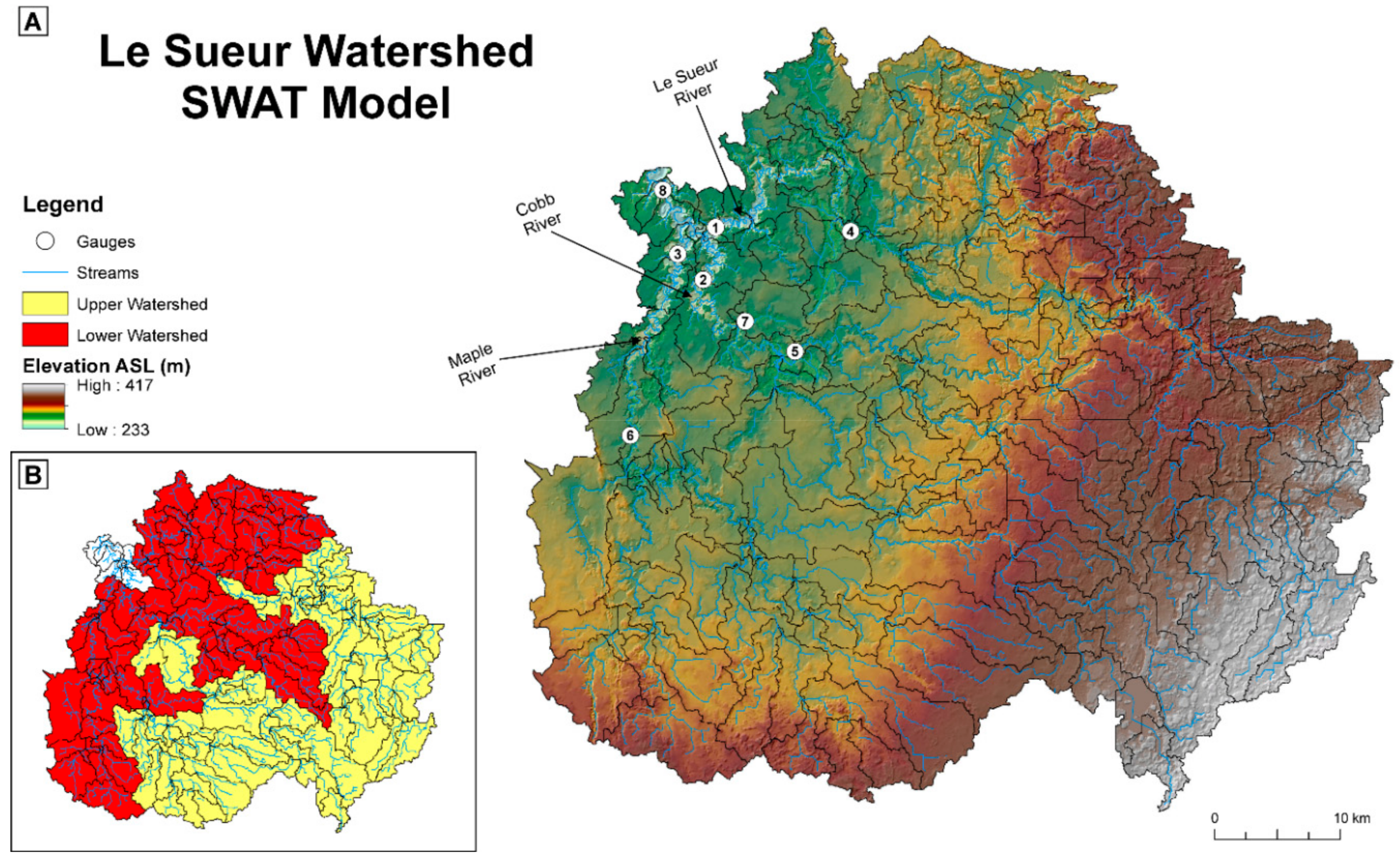
1.1. Background and Study Area

The Minnesota River and many of its tributaries (Figure 1) carry large suspended sediment loads, causing the Minnesota Pollution Control Agency (MPCA) to list over 100 reaches within the MRB as impaired for sediment under Section 303d of the Clean Water Act [15]. Tributaries to the Minnesota River have been among the most rapidly incising rivers in the world throughout the Holocene, as the drainage of glacial Lake Agassiz scoured the mainstem Minnesota River valley starting approximately 13,400 years ago, dropping base level as much as 70 m for tributaries [12,16,17,18,19]. While the uplands of tributary basins have not yet received the signal of base level fall, lower reaches feature knickzones (Figure 1) created as the wave of incision propagates upstream [8,19,20]. Steep, fine-grained till bluffs in the knickzone contribute large quantities of sediment to the channel network [7,21,22,23,24]. This transient adjustment created naturally high sediment-loading rates, but sedimentation records from Lake Pepin, a naturally dammed lake further downstream on the mainstem Mississippi River (Figure 1B), show that sediment loads have increased by an order of magnitude since 1830 CE [25]. Most of this increase originated in the MRB [25,26,27], with the Minnesota River’s contribution to Lake Pepin’s sediment loads increasing from 83.9% (±1.1) to 90.0% (±1.4) [26].

These high sediment loads are related to increases in both stream flows and the erosion rates of near-channel features like stream banks and bluffs [4,7]. Within the MRB, five-year averages of mean annual stream flow, summer and winter low flow, summer peak flow, and flood duration all increased from 1980 to 2014 [5,6,28]. Although some of this hydrologic change has been attributed to climate change [4], local land use changes like artificial drainage have been found to be the main driver [5,29,30,31]. Because the region’s soils are dominated by silts and clays [32], farmers enhance their crop yields with artificial drainage. Ditches and subsurface tiling have connected previously isolated basins to stream networks, effectively increasing some tributaries’ drainage areas by 15–20% [3]. Increased stream flows wield higher shear stresses along bluff toes, causing higher bluff erosion rates [23]. Most eroded bluff material quickly becomes part of a stream’s suspended or wash load, increasing turbidity levels [23]. Indeed, in the Le Sueur watershed, stream banks and bluffs comprise less than 1% of the watershed but provided 70% of the Le Sueur River’s sediment load from 2000 to 2010 [7,33].

1.2. High Flow Attenuation

A potential management strategy for these erosion and sediment loading issues is flood attenuation through water storage structures. Wetland restoration has been widely advocated as a method for flood reduction [34,35,36]. Indeed, Javaheri and Babbar-Sebens [37] used both a hydrologic model, the Soil and Water Assessment Tool (SWAT), and a hydraulic model, the Hydrologic Engineering Center’s River Analysis System (HEC-RAS), to find that wetlands could reduce peak flows, flood areas, and maximum velocities by up to 42%, 55%, and 15%, respectively, within a watershed in central Indiana. In a real-world example, Brody et al. [38] found that wetland alteration in Texas and Florida exacerbated flood events in coastal watersheds. Wetland restoration could also address agricultural pollution [35,36,39,40] in the Le Sueur watershed, but meetings with stakeholders in the region suggest that many are not receptive to installing permanent wetlands but would consider simple detention basins. By focusing only on hydrological considerations here, rather than biochemical or ecological, our intention is to evaluate the flow reduction capacity of generalized water storage structures.

1.3. Research Questions and Approach

This study assesses the potential for a wide range of water retention site (WRS) implementation scenarios to reduce both high flows and sediment-loading rates in an agricultural basin with high near-channel sediment inputs due to postglacial incision, using the Le Sueur River watershed as a case study. This 2800 km² watershed has three gauged rivers we focus on: The Le Sueur, Cobb, and Maple Rivers (Figure 2). We pursue the following research questions: (1) How much can increase water storage reduce high flows? (2) How much can the erosion of near-channel features and subsequent sediment loading be reduced through high flow attenuation? (3) Do high flow reductions from increased water storage follow discernable patterns that could allow for predictability? We use the term “high flows” here for all high magnitude, low exceedance probability stream flows and the term WRS as a general reference for depressional storage areas that could be designed to act as either ecologically functional wetlands or simple detention basins. We vary the extent and placement of WRS within the watershed (e.g., close to or far from the watershed outlet), design depth, and hydraulic conductivity as a proxy for water retention time to test sensitivity to such factors. Projections are made using (1) a widely used watershed-scale hydrological model, SWAT [41], and (2) an empirical sediment-loading relationship for the knickzone of the MRB [13]. Although we use SWAT’s sub-basin-level wetlands to simulate the WRS, the hydrological behaviors used are not specific to wetlands and could apply to detention basins. In addition to projected high flow and sediment loading alterations, we analyzed how high flow reductions scale with WRS extent for different flow exceedance bins, developing a generalized model for flow reductions. This generalization of high flow reductions by distributed water storage can aid in assessing future scenarios rapidly without the use of a model such as SWAT.

2. Methods

2.1. WRS Definition

The WRS used here (Figure 1A) are defined as (1) topographic depressions determined by the difference between filled and unfilled 9-m digital elevation models (DEMs) derived from 3-m lidar data with (2) specific land use types defined by the National Land Cover Database (NLCD) 2011 layers (only barren land, cultivated cropland, hay/pasture, or herbaceous), (3) relatively high compound topographic index (CTI) values, (4) areas over 3000 m², and areas not featuring either (5) sites from the Fish and Wildlife Service’s wetland inventory for the conterminous United States (CONUS) or (6) current conservation easements [13]. The minimum area was selected to limit the number of widely distributed small sites, as feedback from a stakeholder group indicated that farmers would be unlikely to install small WRS that could be obstacles for maneuvering large agricultural equipment. CTI is known as the compound topographic index or topographic wetness index [42], and is calculated as

$$CTI=\ln \left(\frac{A_s}{\tan \beta }\right)$$

(1)

where A_s is the upstream contributing area per unit width (m), where width is orthogonal to flow direction, and β is slope (radians). Prioritizing locations with high CTI values targets sites that are more likely to receive and hold water. All WRS have average CTI values over 11.5 based on previous studies (e.g., [42]). Each site’s volume is defined as the surface area multiplied by the average depression depth. The sites occupy 8.4% of the watershed’s area and the total volumetric capacity of the sites (2.35 × 10⁸ m³) offers about 81 mm of water storage across the watershed. It is important to note that our estimates of potential water storage are conservative, not only because we have limited the types of sites considered, but also because we are only using the natural depressional areas. Water storage volume could most certainly be increased or a similar amount of water could be stored on a smaller footprint if artificial berms and levees were constructed.

2.2. SWAT Model

We used a well-calibrated 2012 SWAT model rev. 637 to predict stream flows for WRS implementation scenarios. SWAT model sub-basins and locations where the model was calibrated are shown in Figure 2. SWAT is an empirically based, semidistributed, and actively used and updated watershed-scale hydrology and water quality model [43]. Parameterization, calibration, and verification of the SWAT model used here are described in greater detail in [44].

Table 1. SWAT model performance metrics for each of the gauges shown in Figure 2, from [44].

Gauge	Number	Cal.	Val.	Cal.	Val.	Cal.	Val.
		NSE		R2		PBIAS
Le Sueur River at Rapidan, CR8	1	0.57	0.75	0.57	0.76	−1.97	1.40
Big Cobb River near Beauford, CR16	2	0.83	0.84	0.84	0.85	3.90	5.03
Maple River near Rapidan, CR35	3	0.72	0.69	0.73	0.7	−21.66	7.85
Le Sueur River at St. Clair, CSAH28	4	0.67	0.72	0.67	0.74	0.25	7.44
Little Cobb River near Beauford	5	0.74	0.79	0.76	0.79	9.90	−2.55
Maple River near Sterling Center, CR18	6	0.72	0.73	0.7	0.75	8.76	17.70
Little Beauford Ditch	7	0.54	0.5	0.55	0.62	17.72	−23.69
Le Sueur River near Rapidan, MN66	8	0.59	0.73	0.6	0.74	15.32	7.67

Note: Cal. and Val. represent the calibration and validation periods, respectively.

shows the model’s performance metrics and

Table 2. List of SWAT model parameters that were calibrated for the Le Sueur watershed, from [44].

Parameter	Description	SWAT Default Value	Calibrated Value
.bsn File—General Watershed Description File
SFTMP	Snowfall temperature (°C)	1	2.2
SMTMP	Snow melt base temperature (°C)	0.5	0.5
SMFMX	Melt factor for snow on 21 June (mm H2O/°C-day)	4.5	4
SMFMN	Melt factor for snow on 21 December (mm H2O/°C-day)	4.5	2
TIMP	Snow pack temperature lag factor	1	0.815
SNOCOVMX	Minimum snow water content that corresponds to 100% snow over (mm H2O)	1	10
SNO50COV	Fraction of snow volume represented by SNOCOVMX that corresponds to 50% snow cover	0.5	0.5
IPET	Potential evapotranspiration (PET) method	Penman/Monteith	Hargreaves
ESCO	Soil evaporation compensation factor	0.95	0.98
EPCO	Plant uptake compensation factor	1	0.005
ICN	Daily curve number calculation method	Soil moisture method	Plant ET method
CNCOEF	Plant evapotranspiration (ET) curve number coefficient	1	0.7
CN_FROZ	Frozen soil infiltration factor	0.000862, ‘inactive’	0.002, ‘active’
ITDRN	Tile drain equation flag	0	1
IWTDN	Water table algorithm flag	0	1
.gw File—Groundwater Input File
GW_DELAY	Groundwater delay time (days)	31	42.63
ALPHA_BF	Baseflow alpha factor (1/days)	0.048	0.83
GWQMN	Threshold depth of water in the shallow aquifer required for return flow to occur (mm H20)	1000	1359.61
GW_REVAP	Groundwater revap coefficient	0.02	0.047
.sub file—Sub-Basin General Input File
CH_N1	Mannings ‘n’ value for tributary channel	0.014	0.04
CH_K1	Effective hydraulic conductivity in tributary channel alluvium (mm/h)	0	30.9
.rte file—Main Channel Input File
CH_N2	Mannings ‘n’ value for main channel	0.014	0.037
CH_K2	Effective hydraulic conductivity in main channel alluvium (mm/h)	0	171.3
.hru file—HRU General Input File
DEP_IMP	Depth to impervious layer in soil profile (mm)	NA	2237.17
RE	Effective radius of drains (mm)	50	25
SDRAIN	Distance between two drains or tile tubes (mm)	NA	NA
OV_N	Manning’s ‘n’ value for overland flow	0.14	0.03

Note: NA—Not Applicable.

shows the parameters that were calibrated and their calibrated values. We evaluated flow reductions at gauges 1–3 in the lower watershed (Figure 2). The daily timestep Nash–Sutcliffe Efficiency (NSE) values for the validation data sets of all gauges except 7 met or exceeded criteria for the highest SWAT performance category defined by [45] (NSE > 0.65; [46]). While gauge 7 had lower NSE values, this gauge only represents the stream flows for one sub-basin and we did not assess results at this gauge.

The model was created using: A 10-m DEM from the United States Geological Survey (USGS) to characterize topography; Cropland Data Layer (CDL) from the year 2006 to specify land use [47]; Soil Survey Geographic Database (SSURGO) soil data [48], 30 years of temperature and precipitation data from the Parameter-elevation Regressions on Independent Slopes Model (PRISM) climate group [49] at 4-km resolution, averaged daily for each sub-basin; and solar radiation and humidity data from global weather data for SWAT [50]. We defined Hydrologic Response Units (HRUs) with the multiple HRUs option, using cutoff thresholds of 5% for land use, 15% for soil, and 10% for slope. The model contained 175 sub-basins and 1823 HRUs. A multipoint and multiparameter calibration was used, and the model was calibrated and validated against daily flows at eight gauges within the watershed (Table 1, Figure 2A). We calibrated flow measurements at gauges using the HydroME Toolbox, moving upstream to downstream, using: (1) NSE, (2) R², (3) Percent bias (PBIAS), and several other metrics discussed by [44]. Each of the WRS scenarios were evaluated with the SWAT model using an automated routine implemented within MATLAB by running 12 simulations in parallel, utilizing all 12 cores of the processor. Each simulation began in 1980 and ended in 2009; output was not recorded for the first five years to allow the model to adjust from initialization errors. More information regarding the model’s development is available in [44].

2.3. Wetland Representation in SWAT

SWAT’s sub-basin-level wetlands were used in this study to simulate the WRS. The water balance of wetlands in SWAT was simulated each day as

$$V_f=V_i+V_{flowin}-V_{flowout}+V_{pcp}-V_{evap}-V_{seep}$$

(2)

where V_f is the final volume of water (m³), V_i is the initial volume (m³), V_flowin is the volume flowing into the wetland from surficial runoff, groundwater, and lateral flow (m³), V_pcp is the volume of direct precipitation (m³), V_evap is the volume evaporated (m³), and V_seep is the volume lost through seepage (m³). See [51] for the equations used to solve each variable in Equation (2).

The V_flowout term in Equation (2) represents overflowing. SWAT allows two overflowing thresholds: The maximum water storage and a lower spilling threshold. When the maximum storage is exceeded, all excess water is spilled. When the lower spilling threshold is used, 1/10 of the excess water above this threshold is spilled each day. Because defining different wetland spilling thresholds that would always satisfy these conditions involves a great deal of uncertainty, this study used only the maximum storage as a spilling threshold so that any excess water was simply spilled. Using a lower spilling threshold tends to provide greater high flow reductions; sites can spill without exceeding their maximum storage, losing more water and having more storage to fill during the next precipitation event.

Wetland behavior in SWAT is sensitive to the K used to solve the V_seep term in Equation (2). The uplands of the Le Sueur watershed are dominated by glacial moraine and lacustrine sediments, as glacial Lake Minnesota covered the western two-thirds of the Le Sueur watershed and left up to 3 m of flat-lying glaciolacustrine silts and clays [12,32]. These sediments offer quite low K values; saturated K values obtained from SSURGO layers [48] are generally on the order of 3.6–36 mm/h (10⁻⁶–10⁻⁵ m/s) in the agricultural uplands. Due to the abundance of silts and clays, the highly variable nature of K over both space and time, the possible accumulation of fine sediment in the sites, and the fact that seepage calculations for SWAT’s wetlands do not consider hydraulic gradients, the scenarios considered in this study used K values within a range of 0.036–3.6 mm/h (10⁻⁸–10⁻⁶ m/s). Although this range does not extend to the highest values shown by SSURGO layers (~36 mm/h) [48], we will show in our results (Section 3) that (1) scenarios using K values of 0.36 or 3.6 mm/h provide similar flow reductions and (2) increased volumetric capacity via design depth has little effect when K = 3.6 mm/h, so higher K values (>3.6 mm/h) would not produce drastically different results. Modified K values do not necessarily imply that humans would alter the soil properties at each site. Rather, K is a simple and reasonable variable to represent drainage rate, which could also be controlled via engineered outlets.

The coefficient used to scale actual evaporation relative to potential evaporation was set to 1 here, rather than the SWAT default value of 0.6. This decision was motivated in part by the lack of simulated plants within SWAT’s wetlands. The differences in wetland behavior caused by this adjustment are slight and only noticeable when K values are very low (e.g., 0.036 mm/h).

The “WET_FR” input parameter (contributing area to all wetlands in a sub-basin/sub-basin area) was used to solve the V_flowin parameter in Equation (2). Despite the parameter’s significant influence on wetland behavior, many studies employing wetlands in SWAT do not sufficiently explain their assumptions regarding contributing areas (e.g., [52,53,54]). Here, we defined WET_FR by (1) manually measuring contributing areas at the farthest downstream outlets of delineated WRS (i.e., all locations where flow accumulation paths exit the WRS in Figure 1A and these paths do not lead to other WRS further downstream) and subtracting the surface areas of the WRS and (2) using regressions of these manual contributing-area measurements to define generalized contributing-area relationships. Because the 175-sub-basin SWAT model used here is finely resolved, we manually measured contributing areas for a coarser sub-basin delineation. The 30 sub-basins used are shown in the Supplementary Information (SI) (Figure S1). During the manual measurements, the extents of delineated WRS (Figure 1A) were varied by prioritizing sites with large surface areas; we selected the largest sites first and added smaller sites as extents increased. This decision was motivated by feedback from a stakeholder group (previously mentioned in Section 2.1) suggesting farmers would be unlikely to install many small sites and may prefer fewer large sites. The contributing-area relationship created with regressions of our manual measurements allowed us to calculate WET_FR in our 175-sub-basin SWAT model, and this relationship could also be utilized in similar geomorphic and climatic regimes.

2.4. WRS Implementation Scenarios

WRS implementation scenarios were created with different combinations of WRS placement in the watershed, design depth, and K. We assessed design depths of 0.5, 1, and 2 m and K values of 0.036, 0.36, and 3.6 mm/h (10⁻⁸, 10⁻⁷, and 10⁻⁶ m/s). Placement scenarios were defined by grouping sub-basins based on their general proximity to the watershed outlet (Figure 2B and Figure S1) because travel distance was expected to influence desynchronization of the hydrograph. Three placement scenarios are used: The entire watershed, upper watershed, or lower watershed (Figure 2B).

2.5. Flow-Reduction Assessment

Discharges occurring at gauges in the knickzone (Figure 1 and Figure 2) were used to assess high flows. Each river has an “upper” gauge situated upstream of the watershed’s knickzone (gauges 4–6) and a “lower” gauge situated within the knickzone (gauges 1–3). We assessed flow reductions at the lower gauges as the vast majority of channel erosion occurs within the geologically unstable knickzone.

We separated flows into groups defined by the flows’ exceedance probabilities (relative to all flows over the 25 years assessed). These exceedance probability bins were spaced logarithmically to highlight the large reductions in high-magnitude flows. Because 90% of all flows occur between the exceedance probabilities of 10–100%, we divided this bin into two smaller logarithmically spaced bins (10–32% and 32–100%). Within each bin, we assessed the slope of the average discharge reduction (relative to the baseline scenario) versus WRS extent using a fixed intercept of 0. Flow-reduction slopes were then evaluated relative to exceedance probability in order to derive generalized relationships between WRS extent and flow reduction for a given exceedance probability.

2.6. Sediment Loading Assessment

Rivers within the MRB experience a sharp increase in sediment loading as they flow through the knickzone, reflecting the erosion of near-channel features such as bluffs [7,33]. Cho [13] developed an empirical relationship between discharges at lower gauges and the near-channel sediment-loading rates for the incised reaches between the upper and lower gauges on multiple rivers within the MRB (including the Le Sueur, Cobb, and Maple Rivers).

The sediment loading from incised reaches is calculated as [13]

$$S=\frac{1}{N}{\displaystyle \sum }L\alpha {\left(\frac{Q}{A_{LG}}\right)}^{\beta } \mathrm{for}\frac{Q}{A_{LG}}> 1 \mathrm{mm}/\mathrm{day}$$

(3)

where S is the sediment added by near-channel features in the incised reach (Mg/yr), Q/A_LG is drainage-area normalized discharge (mm/day) at a lower gauge and exceeding the threshold of 1 mm/day, L is the length of the incised channel between the upper and lower gauges (40.84, 31.91, and 35.79 km for the Le Sueur, Cobb, and Maple), N is the number of years evaluated, and 𝛼 and 𝛽 are 0.5386 and 2.137, respectively [13]. For all WRS implementation scenarios, S values were normalized by the corresponding S value in the baseline scenario (i.e., no WRS used) and referred to as S’, with a subscript denoting the location (S_L’, S_C’, and S_M’ for the lower gauges on the Le Sueur, Cobb, and Maple). It is worth noting that Equation (3) was derived using 15-min discharge data, but SWAT provides only daily mean discharge values. Because daily flows underestimate flood peaks, sediment loads for daily flows using Equation (3) tend to be underpredicted. To account for this, we only compared sediment loading results from different scenarios relative to baseline conditions rather than absolute load reductions.

3. Results

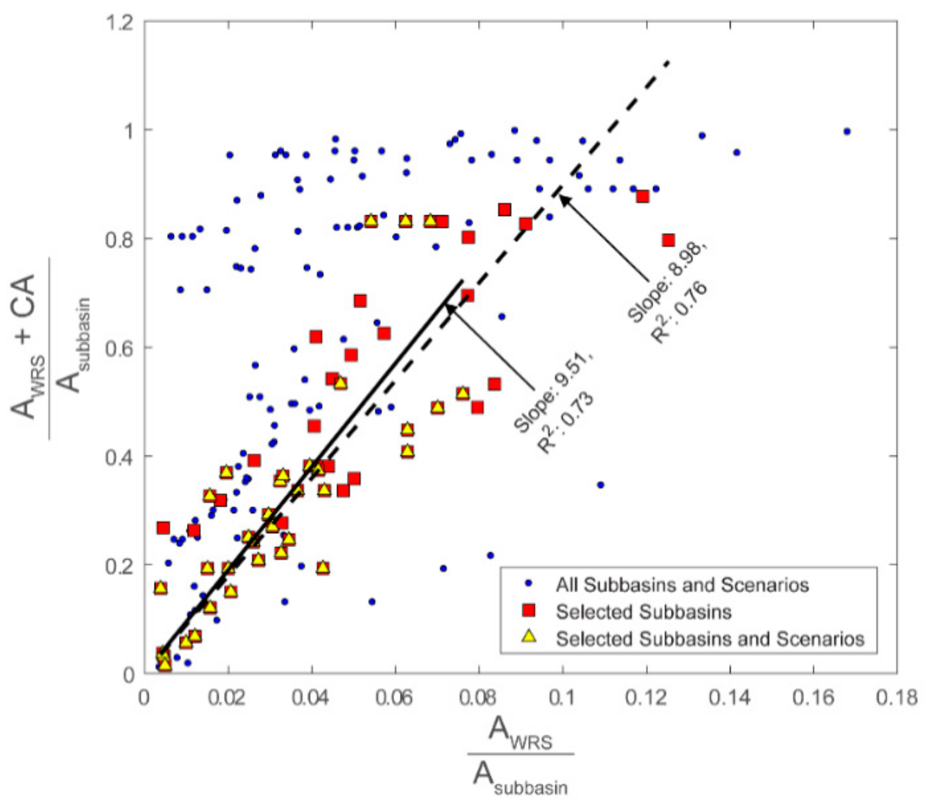
3.1. Contributing-Area Relationships

Regressions of our contributing-area (CA) measurements for delineated WRS (Figure 1A) allowed us to solve for SWAT’s WET_FR parameter (Figure 3), removing the constraint of manually measuring CA for our WRS scenarios. Obtaining an equation for WET_FR as a function of CA, however, required us to refine our selection. Measurements for all sub-basins (Figure S1) include considerable scatter (blue circles in Figure 3). Much of this scatter is caused by natural depressions situated along channel networks in the low-gradient uplands (Figure S2). With WRS situated on main channels, there are abrupt and unpredictable changes in CA. For example, placing even one site on a main channel could cause CA values to increase dramatically and remain high at subsequent extents (blue circles with high (A_WRS + CA)/A_subbasin at low extents in Figure 3). Excluding the data for sub-basins with WRS on main channels yields a linear trend (red squares in Figure 3). These data level off at high WRS extents (about 8%). Given that such high WRS extents are unlikely to be implemented, these higher extents were also removed (yellow triangles in Figure 3), yielding a simple linear regression where CA = 8.51A_WRS. WET_FR is then CA/A_subbasin, and we evaluated A_WRS/A_subbasin values of 0.5%, 1%, 2%, 4%, and 7.5% in our WRS scenarios. Note that (1) the y-axis of Figure 3 is $\frac{CA+A_{WRS}}{A_{subbasin}}$ rather than $\frac{CA}{A_{subbasin}}$, making CA = 8.51A_WRS, (2) avoiding sub-basins with WRS situated on main channels (Figure S2) likely makes our CA estimates conservative, and (3) excluding high WRS extents (yellow triangles in Figure 3) pertains to prioritizing by surface site area (Section 2.3) rather than simply imposing a limit on A_WRS/A_subbasin (i.e., since WRS with large surface areas were prioritized, the higher WRS extents excluded were adding WRS with smaller surface areas).

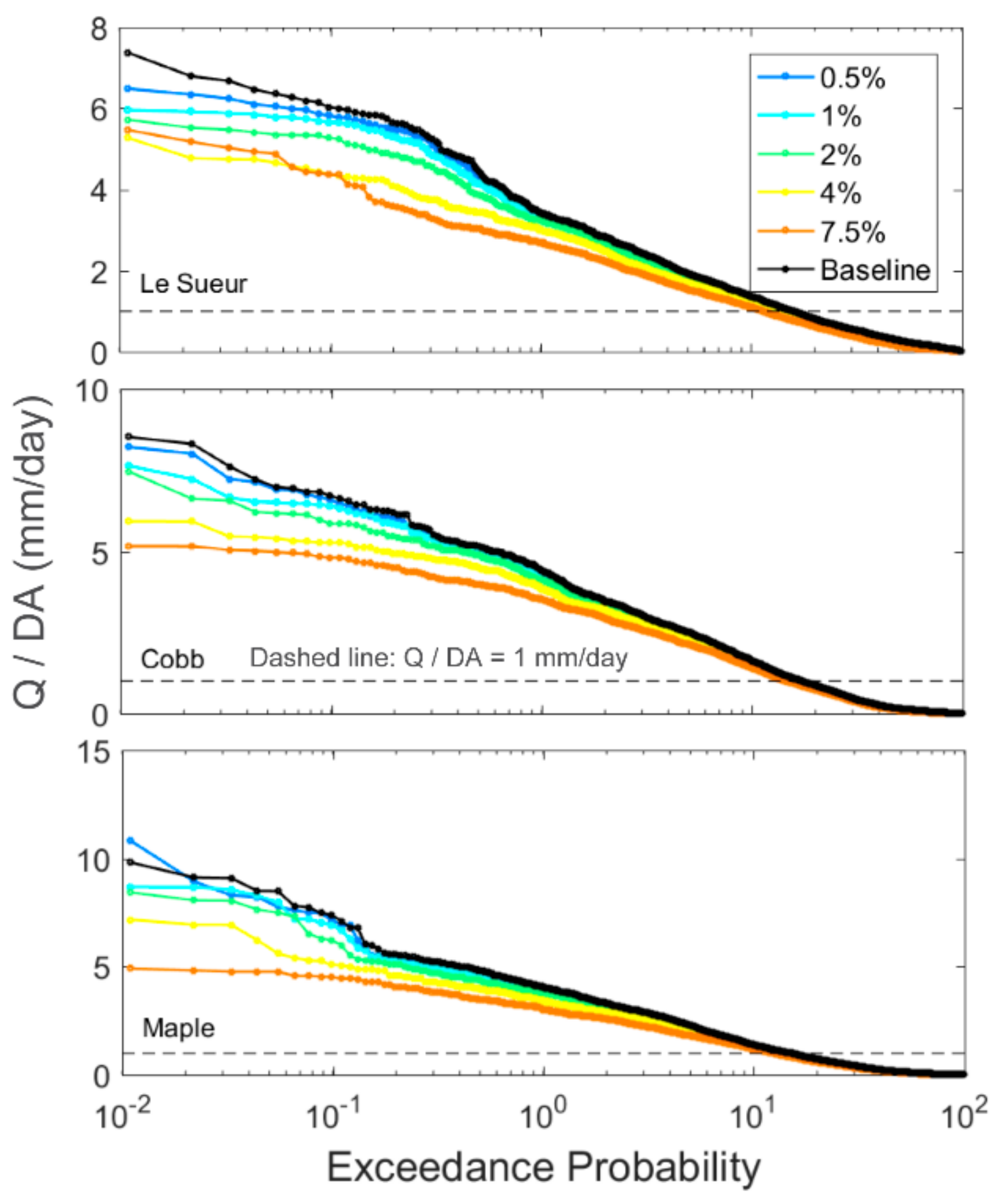
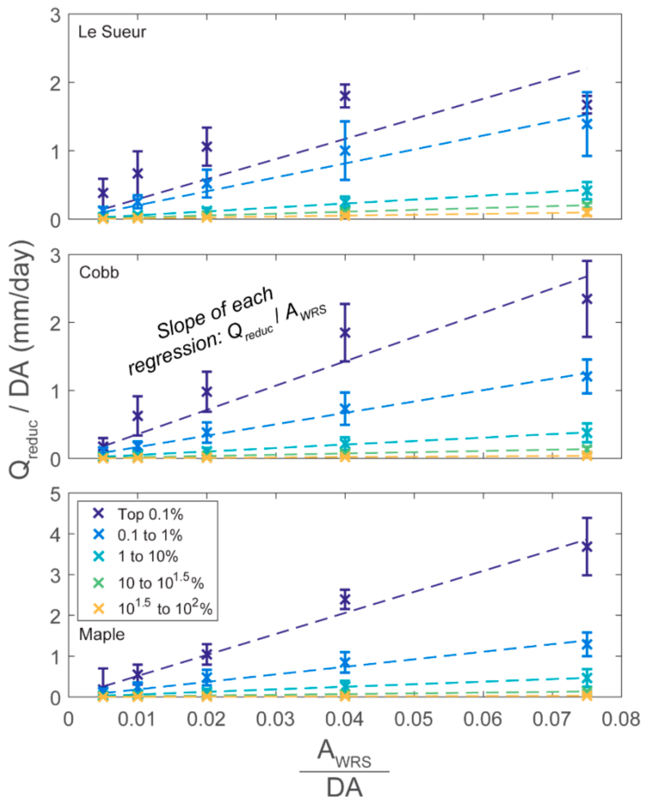
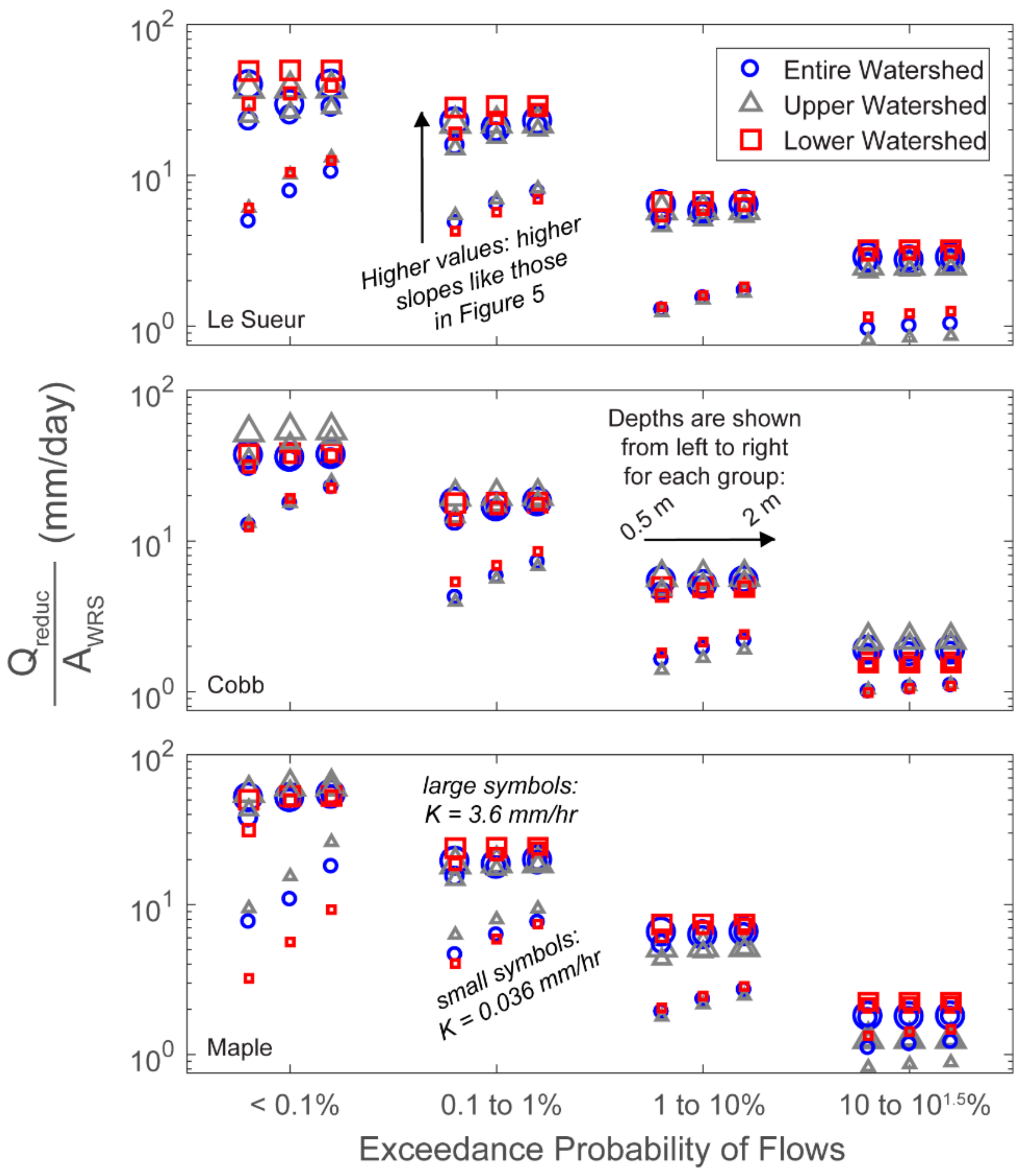
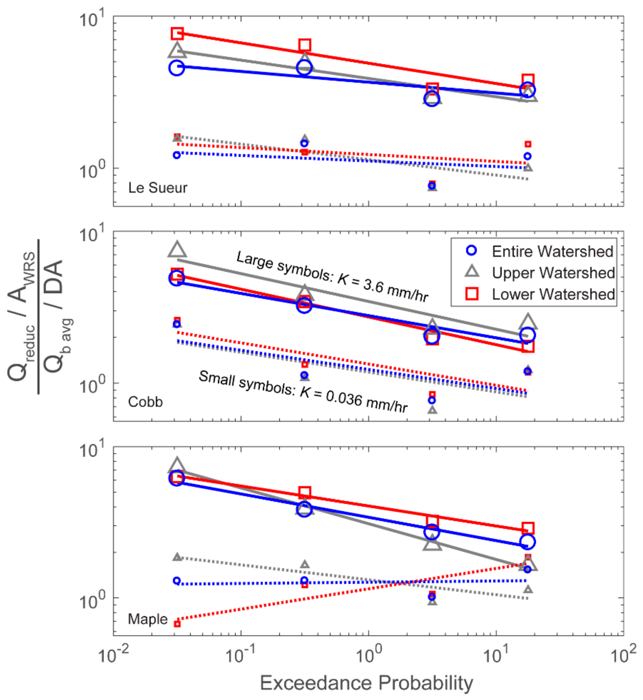
3.2. Flow Reductions

Figure 4 shows an example of the flow reductions offered by WRS scenarios. Here, WRS were placed throughout the entire watershed, depths of 1 m were used, and K = 3.6 mm/h. With few exceptions, high flows tend to gradually decrease with increasing WRS extent. The highest reductions are achieved within the top 1% of flows, while the sediment-loading threshold of 1 mm/day occurs at exceedance probabilities between 10% and 20% (Figure 4).

Flow reduction as a function of WRS extent can be reasonably approximated via linear regression. We evaluated linear regressions for each log-bin of exceedance probabilities, for flows at gauges 1–3 in the lower watershed (Figure 2A), comprising a total of 405 regressions across all scenarios. All regressions have intercepts fixed at the origin. Figure 5 shows three regression analyses, as examples. Flow reductions are shown as Q_reduc/DA, which represents the average reduction for each flow bin’s normalized discharge values. The slope of each regression is Q_reduc/A_WRS. Virtually all regressions had R² > 0.9, except four of the regressions for the top 0.1% of flows. Of these four regressions, one was for the Le Sueur, with R² = 0.74; this scenario used WRS placement throughout the entire watershed, design depths of 1 m, and K = 3.6 mm/h (Figure 5). The three other regressions were for the Maple with R² values of 0.34, 0.55, and 0.74 for depths of 0.5, 1, and 2 m with K = 0.036 mm/h and placement in the lower watershed. These poor regressions for the top 0.1% of flows generally cause flow reductions to be underpredicted for low WRS extents (<4%) and slightly overpredicted for the highest WRS extents (7.5%) but are notably only 4 of the 81 regressions (~5%) for the top 0.1% of flows. These linear regressions are generally representative of flow reductions and, quite importantly, allow for comparison between all flow groups. In contrast, regressions with varying nonlinearities could not be compared directly. All regressions are available in Tables S1–S15.

Flow reductions for all WRS scenarios are summarized in Figure 6. Because we focus on high flows here, results for the exceedance-probability bin of 32%–100% are not shown in Figure 6 but are available in the SI. For each exceedance-probability bin in Figure 6, the left, center, and right values correspond with design depths of 0.5, 1, and 2 m, respectively. Each depth then has 3 K scenarios for 3 WRS placement scenarios (placement in entire, upper, and lower watershed). K values are represented by symbol size, with small, medium, and large symbols for K = 0.036, 0.36 and 3.6 mm/h, respectively. In general, K values are the most sensitive factor influencing WRS performance. Higher seepage rates allow the WRS to lose more water between events, enabling them to intercept more of the next event’s water and attenuate high flows. The separation in site performance between K values of 0.036 and 0.36 mm/h is larger than that between 0.36 and 3.6 mm/h. Design depths have a larger impact for lower K values. Because the addition of WRS capacity via design depth has no apparent effect when K is 3.6 mm/h, the sites seem to be handling all water input without increases in overflowing. Our results do not suggest WRS placement is a first-order control on site behavior in this watershed; different placement scenarios are only slightly better for different subwatersheds (e.g., upper watershed for the Cobb and lower for the Le Sueur in Figure 6). These differences are not significant enough to draw generalized conclusions regarding site placement.

When flow-reduction slopes (Q_reduc/A_WRS; Figure 5 and Figure 6) are (1) placed at the center of their corresponding bin (10^−1.5%, 10^−0.5%, 10^0.5%, 10^1.25%) and (2) normalized by the average baseline discharge for that bin (Q_{b avg}/DA; Table S16), they exhibit a power-law scaling with exceedance probability (Figure 7). Results for K = 0.36 mm/h are not shown in Figure 7 because of their similarity to those for K = 3.6 mm/h, but they are available in the SI. Regressions fit to baseline-normalized flow-reduction slopes allow the flow for any exceedance probability to be predicted as a function of WRS extent:

$$Q_{sim}=Q_b\left(1-\gamma P^{\epsilon }\frac{A_{WRS}}{DA}\right)$$

(4)

where Q_sim is the simulated, normalized discharge (mm/day), Q_b is the baseline discharge normalized by drainage area for the given exceedance probability (mm/day), P is the exceedance probability considered, $\gamma$ is a coefficient, ε is an exponent, A_WRS is the upstream WRS area (m²), and DA is the drainage area where flows are evaluated (m²). Note that $\gamma$P^ε represents the P vs. $\frac{\raisebox{1ex}{$Q_{reduc}$}\!\left/ \!\raisebox{-1ex}{$A_{WRS}$}\right.}{\raisebox{1ex}{$Q_{b avg}$}\!\left/ \!\raisebox{-1ex}{$DA$}\right.}$ regressions shown in Figure 7, and that multiplying these values by $Q_b\frac{A_{WRS}}{DA}$ yields a scaled $Q_{reduc}$ value. These relationships reproduce results from our well-calibrated SWAT model quite accurately (Figure 8, Figures S5 and S6), instilling confidence that they may be applicable to other settings. Because we focus on high flows, the bin with the lowest flows (exceedance probability >32%) was not included in these regressions. The $\gamma$ε, and R² values of all regressions are available in Tables S17–S19. R² values generally increase with K. Scenarios with K = 3.6 mm/h always have R² > 0.82, except for one scenario for the Le Sueur (R² = 0.67 for depths of 1 m and placement throughout the entire watershed). Scenarios with K = 0.036 or 0.36 mm/h have highly variable R² values. Across all K, depth, and placement scenarios, regressions with high R² values generally have 𝜀 ranging from about −0.2 to −0.1 and γ ranging from about 2 to 4 (Figures S3 and S4). Scenarios with higher K values tend to have higher γ and ε lower values, but a generally representative parameter set for a high R² scenario is ε = −0.15 and γ = 3 (Figure S4). Despite the lower R² values of some of these regressions, results for scenarios using depths of 1 m and K = 0.036 or 0.36 mm/h are still predicted quite accurately (Figures S5 and S6). These generalized high flow-reduction relationships may allow for rapid scenario testing without the use of models like SWAT.

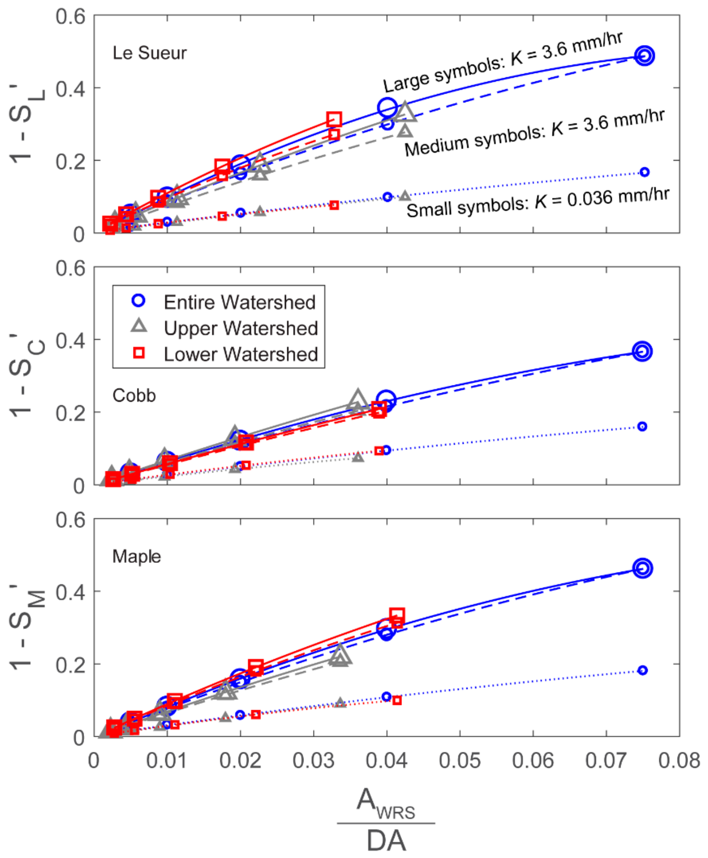
3.3. Sediment-Loading Reductions

Our results suggest that sediment loading from near-channel sources like bluffs can be substantially reduced through high flow reduction (Figure 9, Figures S7 and S8). In Figure 9, scenarios for all K values and site placements are shown for 1-m design depth scenarios. In our highest WRS extents (7.5% basin area in WRS), sediment inputs above the threshold can be reduced by over 40% in the Le Sueur and Maple Rivers and just under 40% in the Cobb River. Again, K values are the most important factor, while site placement does not seem to be as significant. Design depths of 2 m reduce the separation between scenarios with higher and lower K values (Figure S8). Depths of 0.5 m increase this separation, although scenarios with K = 0.036 mm/h and depths of 0.5 m provide only slightly lower sediment-loading reductions than those in Figure 8 (Figure S7).

When compared against sediment budgets for the Le Sueur watershed [7,33,55], sediment-loading rates computed from Equation (3) using SWAT-derived daily flow data for each incised reach are underpredicted (

Table 3. Mud input between the upper and lower gauges on each of three study rivers.

Source	Mud Input (Mg/yr) between the Upper and Lower Gauges
	Le Sueur	Cobb	Maple
Sediment Budget 2000–2010, v2 1	2.85 × 104	2.76 × 104	2.34 × 104
Sediment Budget 2000–2010, v1 1	2.47 × 104	2.44 × 104	2.08 × 104
15-min Flows 2006–2011, Gauged 2	2.34 × 104	2.46 × 104	3.04 × 104
Daily Flows 2005–2009, Gauged 2	6.05 × 103	4.97 × 103	6.41 × 103
Daily Flows 2005–2009, SWAT 3	6.46 × 103	7.63 × 103	7.24 × 103
Daily Flows 1985–2009, SWAT 3	6.58 × 103	7.60 × 103	7.44 × 103

¹ Sediment budget v1 (from [7,33]) was used in validation of the sediment-loading model by [13] (Equation (3)). Sediment budget v2 was updated by Bevis [55]. Loads here only include erosion from near-channel sources (bluffs and streambanks). ² Comparison of sediment loads predicted by sediment-loading model of [13] using 15-min and daily data from flow gauges. Gauged daily flows for the Le Sueur River are limited to 2006–2009. ³ Prediction sediment loads using sediment-loading model of [13] and daily flows in SWAT model used for this analysis. For 2005–2009, SWAT-projected flows were only used on days with gauged flows available.

). This difference is due in part to Equation (3) having been derived using 15-min discharge data rather than the daily mean flows produced by SWAT; sediment-loading rates calculated from gauged 15-min discharge data are more accurate (Table 3). Sediment-loading rates calculated from SWAT flows, however, closely match those calculated from gauged daily mean flows (Table 3; gauged vs. SWAT modeled daily flows in Figure S9). Because of the potential for underpredicting loads with daily time-step data, sediment reduction results here are all presented relative to the baseline SWAT scenario.

4. Discussion

Our results show that distributed water storage can be an effective practice for reducing high flows and therefore erosion of near-channel sediment sources. While the sediment reduction potential may be amplified in our study basin, due to the geologically unstable knickzones, water storage should be expected to provide substantial sediment reduction in the many watersheds that have experienced substantial anthropogenic increases in flows [29]. These findings agree with those of other studies, which also used SWAT’s wetland functionality to show that wetland restoration decreases stream flows in both prairie regions of Manitoba, Canada [53,56] and northwestern Minnesota [53]. Although Martinez-Martinez et al. [54] found wetland restoration to offer minimal flow reductions in an agricultural watershed in central Michigan, their flow-reduction metrics (long-term average daily streamflow, daily peak flows, frequency of peak flow events) and wetland restoration scenarios (placement in only one sub-basin per simulation, restored wetland areas only up to 0.17% of watershed area) differ substantially from those considered in our study.

We found the most important factor in site performance is K, with higher K values providing higher flow reductions across the range tested here. This result may seem counterintuitive, as increased hydraulic conductivity via tile drainage is thought to have increased high flows [4]. In the case of tile drainage, however, water seeping into the ground can reach a stream within minutes to hours [57], moving through pipes and bypassing the groundwater flow that would otherwise be required. In contrast, water seeping through the bottom of a WRS would move through shallow groundwater and then to the channels, taking considerably longer. The SWAT wetlands used here to simulate WRS only lose water in three ways: (1) evaporation, (2) overflowing, and (3) seepage. We did not alter either (1) wetland evaporation rates, by changing the parameter that scales wetlands’ evaporation rates between different simulations, or (2) overflowing behavior by using lower spilling thresholds. Setting a lower spilling threshold allows wetlands to lose more water and have more storage available for upcoming precipitation events. We did not use a lower spilling threshold, and our flow reductions may be conservative as a result. Because we focused on varying K, our scenarios highlight K’s role in enhancing seepage and preventing overflowing. Our results suggest that spatially distributed water storage structures with K values of 0.36–3.6 mm/h are more effective. Real WRS installed in the landscape may utilize control structures to mimic drainage rates similar to the range of K values simulated here.

The approach used here for assessing flow reductions provides robust and simple metrics that can be compared across scenarios, but by virtue of its simplicity, avoids certain details that are worth discussing. Flows within each exceedance probability bin do not always monotonically decrease with WRS extent; reducing one flood might cause it to enter another probability bin, potentially offsetting some of that bin’s flow reductions. Alternatively, WRS may attenuate one precipitation event but overflow during the next event due to already high water storage, potentially increasing the second event’s flows relative to the baseline scenario. Such details are lost in this lumped binning approach. Our approach for computing flow reduction via linear regression against WRS extent generally worked well, however, with 99% of the regressions achieving R² > 0.9 (Tables S1–S15). Our generalized relationships between flow exceedance probabilities, flow reductions, and WRS extent (Figure 7 and Figure 8) accurately reproduced results from our well-calibrated SWAT model, which instills some confidence that these generalized relationships may be applicable to real, observed flow duration curves for areas geomorphically and climatically similar to the Le Sueur watershed.

While SWAT is a powerful tool, there are issues with SWAT’s treatment of wetlands. The lumping of all wetlands within each sub-basin in a SWAT model can allow for unrealistic behaviors. For example, water is redistributed amongst all wetlands in a sub-basin, regardless of their distance or orientation with each other. We do not attempt to portray actual sites here, only realistic total storage volumes, and our contributing-area relationship applies to lumped sites distributed throughout a sub-basin. We have also attempted to err substantially on the conservative side in estimating realistic total storage volumes such that potentially larger volumes of water could be stored in a smaller fraction of the watershed, especially if berms and levees are constructed. While we do not expect this issue to have substantially biased our results, lumping wetlands at the sub-basin scale remains an issue that should be reconciled in future versions of SWAT. For example, each sub-basin could have multiple wetlands with individualized storages and contributing areas. Otherwise, studies employing SWAT’s sub-basin-level wetlands should ensure that this depiction is suitable for the wetlands they intend to represent (e.g., better for fewer, larger wetlands and not as appropriate for many small wetlands situated far from each other within a large sub-basin).

One might expect site placement to have a stronger effect on flow reductions than our results suggest (Figure 6). For example, Martinez-Martinez et al. [54] found wetland placement in SWAT to influence flow reductions in an agricultural watershed in central Michigan. Their results generally showed wetland placement in the upper watershed to be more effective at decreasing flows at the watershed outlet (Figure 14a in [54]), but as stated previously, their wetland restoration scenarios are quite different from those assessed here. If site placement is not a first-order control on site performance, as shown by our results, then interested parties can prioritize low-cost areas situated throughout the watershed. We did create our contributing-area relationship by prioritizing depressions with high CTI (topographic wetness index) values, however, and real sites should still be optimally located to receive and hold water.

Our results suggest that WRS can be an effective management option for the reduction of erosion and sediment loading in incised agricultural watersheds like the Le Sueur (Figure 9). Maintaining WRS may be costly, with costs ranging from a few hundred dollars to tens of thousands of dollars per acre-foot, for a simple berm-detention basin to a functioning, created wetland, respectively (e.g., [58]). Nevertheless, these costs must also be compared with the costs and expected lifetimes of other management options. Furthermore, WRS can also provide additional ecosystem services, such as habitat and the interception and treatment of excess nutrients [35,36,39,40,56,59,60]. An effective management strategy will likely target high priority, easily accessed bluffs while also weighing the benefits of increased water storage [61], but that full cost-benefit analysis goes well beyond the scope of this study.

5. Conclusions

Constructed water storage sites distributed throughout a watershed can reduce high flows and, consequently, sediment loading from near-channel sediment sources. We present relationships between WRS contributing areas and WRS extent that allow for flexibility in assessing scenarios over a range of design depths and site placement strategies in the Le Sueur watershed. Site performance depends primarily on K because of its role in enhancing seepage and reducing overflowing. We note that we used K as a means to control drainage of the WRS. While K is not easily manipulated over large spatial scales, our simulations are on the low end for K’s mapped throughout the watershed and engineered structures could be utilized to attain whatever drainage rate is needed at each individual site. The key point is that optimal solutions detain water sufficiently long to desynchronize the high flows downstream but drain sufficiently rapidly to have storage capacity available for the next rainfall event. Higher design depths can enhance flow reductions from sites with low K values. Results have only slight differences between different site placement scenarios (e.g., entire watershed vs. upper or lower), suggesting site placement is not a first-order control on site performance in this watershed. Flow reductions in our SWAT model exhibit a power-law scaling with exceedance probability that enable generalized flow-reduction relationships. These relationships accurately reproduce our results and may be applicable to real flow duration curves.

References

1. Dahl, T.E.; Allord, G.J. History of wetlands in the conterminous United States. In National Summary on Wetland Resources; United States Geological Survey (USGS) and the US Government Printing Office: Washington, DC, USA, 1996; pp. 19–26. [Google Scholar]
2. Blann, K.L.; Anderson, J.L.; Sands, G.R.; Vondracek, B. Effects of agricultural drainage on aquatic ecosystems: A review. Crit. Rev. Environ. Sci. Technol. 2009, 39, 909–1001. [Google Scholar] [CrossRef]
3. Lenhart, C.F.; Verry, E.S.; Brooks, K.N.; Magner, J.A. Adjustment of prarie pothole streams to land-use, drainage, and climate changes and consequences for turbidity impairment. River Res. Appl. 2012, 28, 1609–1619. [Google Scholar] [CrossRef]
4. Schottler, S.P.; Ulrich, J.; Belmont, P.; Moore, R.; Lauer, J.W.; Engstrom, D.R.; Almendinger, J.E. Twentieth century agricultural drainage creates more erosive rivers. Hydrol. Process. 2014, 10, 1951–1961. [Google Scholar] [CrossRef]
5. Kelly, S.; Takbiri, Z.; Belmont, P.; Foufoula-Georgiou, E. Human amplified changes in precipitation-runoff patterns in large river basins of the Midwestern United States. Hydrol. Earth Syst. Sci. 2017, 21, 5065. [Google Scholar] [CrossRef]
6. Novotny, E.V.; Stefan, H.G. Stream flow in Minnesota: Indicator of climate change. J. Hydrol. 2007, 334, 319–333. [Google Scholar] [CrossRef] [Green Version]
7. Belmont, P.; Gran, K.B.; Schottler, S.P.; Wilcock, P.R.; Day, S.S.; Jennings, C.; Lauer, J.; Viparelli, E.; Willenbring, J.; Engstrom, D.; et al. Large shift in source of fine sediment in the Upper Mississippi River. Environ. Sci. Technol. 2011, 45, 8804–8810. [Google Scholar] [CrossRef] [PubMed]
8. Gran, K.B.; Belmont, P.; Day, S.S.; Finnegan, N.; Jennings, C.; Lauer, J.W.; Wilcock, P.R. Landscape evolution in south-central Minnesota and the role of geomorphic history on modern erosional processes. GSA Today 2011, 21, 7–9. [Google Scholar] [CrossRef]
9. Lauer, J.W.; Echterling, C.; Lenhart, C.; Belmont, P.; Rausch, R. Air-photo based change in channel width in the Minnesota River basin: Modes of adjustment and implications for sediment budget. Geomorphology 2017, 297, 170–184. [Google Scholar] [CrossRef]
10. Belmont, P.; Foufoula-Georgiou, E. Solving water quality problems in agricultural landscapes: New approaches for these nonlinear, multi-process, multi-scale systems. Water Resour. Res. 2017, 53, 2585–2590. [Google Scholar] [CrossRef]
11. Lenhart, C.F.; Smith, D.J.; Lewandowski, A.; Belmont, P.; Gunderson, L.; Nieber, J.L. Assessment of Stream Restoration for Reduction of Sediment in a Large Agricultural Watershed. J. Water Resour. Plan. Manag. 2018, 144, 04018032. [Google Scholar] [CrossRef]
12. Gran, K.B.; Finnegan, N.; Johnson, A.L.; Belmont, P.; Wittkop, C.; Rittenour, T. Landscape evolution, valley excavation, and terrace development following abrupt postglacial base level fall. Geol. Soc. Am. Bull. 2013, 125, 1851–1864. [Google Scholar] [CrossRef]
13. Cho, S.J. Development of Data-Driven, Reduced-Complexity Watershed Simulation Models to Address Agricultural Non-Point Source Sediment Pollution in Southern Minnesota. Ph.D. Thesis, John Hopkins University, Baltimore, MD, USA, 2017. [Google Scholar]
14. Vaughan, A.A.; Belmont, P.; Hawkins, C.P.; Wilcock, P. Near-Channel Versus Watershed Controls on Sediment Rating Curves. J. Geophys. Res. Earth Surf. 2017, 122, 1901–1923. [Google Scholar] [CrossRef]
15. Minnesota Pollution Control Agency Minnesota’s Impaired Waters List. 2014. Available online: http://www.pca.state.mn.us/index.php/water/water-types-and-programs/minnesotas-impaired-waters-and-tmdls/impaired-waters-list.html (accessed on 4 August 2018).
16. Matsch, C.L. River Warren, the southern outlet to glacial Lake Agassiz. Glacial Lake Agassiz 1983, 26, 231–244. [Google Scholar]
17. Thorleifson, L.H. Review of Lake Agassiz history. Sedimentol. Geomorphol. Hist. Cent. Lake Agassiz Basin Geol. Assoc. Can. Field Trip Guideb. B 1996, 2, 55–84. [Google Scholar]
18. Fisher, T.G. Chronology of glacial Lake Agassiz meltwater routed to the Gulf of Mexico. Quat. Res. 2003, 59, 271–276. [Google Scholar] [CrossRef]
19. Belmont, P. Floodplain width adjustments in response to rapid base level fall and knickpoint migration. Geomorphology 2011, 128, 92–102. [Google Scholar] [CrossRef]
20. Gran, K.B.; Belmont, P.; Day, S.S.; Jennings, C.; Johnson, A.; Perg, L.; Wilcock, P.R. Geomorphic evolution of the Le Sueur River, Minnesota, USA, and implications for current sediment loading. Manag. Restor. Fluv. Syst. Broad Hist. Chang. Hum. Impacts: Geol. Soc. Am. Spec. Pap. 2009, 451, 119–130. [Google Scholar] [CrossRef]
21. Sekely, A.C.; Mulla, D.J.; Bauer, D.W. Streambank slumping and its contribution to the phosphorus and suspended sediment loads of the Blue Earth River, Minnesota. J. Soil Water Conserv. 2002, 57, 243–250. [Google Scholar]
22. Kelly, S.A.; Belmont, P. High Resolution Monitoring of River Bluff Erosion Reveals Failure Mechanisms and Geomorphically Effective Flows. Water 2018, 10, 394. [Google Scholar] [CrossRef]
23. Day, S.S.; Gran, K.B.; Belmont, P.; Wawrzyniec, T. Measuring bluff erosion part 2: Pairing aerial photographs and terrestrial laser scanning to create a watershed scale sediment budget. Earth Surf. Process. Landf. 2013, 38, 1068–1082. [Google Scholar] [CrossRef]
24. Schaffrath, K.R.; Belmont, P.; Wheaton, J.M. Landscape-scale geomorphic change detection: Quantifying spatially variable uncertainty and circumventing legacy data issues. Geomorphology 2015, 250, 334–348. [Google Scholar] [CrossRef] [Green Version]
25. Engstrom, D.R.; Almendinger, J.E.; Wolin, J.A. Historical changes in sediment and phosphorus loading to the upper Mississippi River: Mass-balance reconstructions from the sediments of Lake Pepin. J. Paleolimnol. 2009, 41, 563–588. [Google Scholar] [CrossRef]
26. Kelley, D.W.; Nater, E.A. Historical sediment flux from three watersheds into Lake Pepin, Minnesota, USA. J. Environ. Qual. 2000, 29, 561–568. [Google Scholar] [CrossRef]
27. Wilcock, P.R. Identifying Sediment Sources in the Minnesota River Basin; Minnesota Pollution Control Agency (MPCA): St. Paul, MN, USA, 2009; Available online: https://www.pca.state.mn.us/sites/default/files/wq-b3-43.pdf (accessed on 4 August 2018).
28. Call, B.; Belmont, P.; Schmidt, J.C.; Wilcock, P.R. Changes in Floodplain Inundation under Non-Stationary Hydrology for an Adjustable, Alluvial River Channel. Water Resour. Res. 2017, 53, 3811–3834. [Google Scholar] [CrossRef]
29. Foufoula-Georgiou, E.; Takbiri, Z.; Czuba, J.A.; Schwenk, J. The change of nature and the nature of change in agricultural landscapes: Hydrologic regime shifts modulate ecological transitions. Water Resour. Res. 2015, 51, 6649–6671. [Google Scholar] [CrossRef] [Green Version]
30. Belmont, P.; Stevens, J.R.; Czuba, J.A.; Kumarasamy, K.; Kelly, S.A. Comment on “Climate and agricultural land use change impacts on streamflow in the upper midwestern United States,” by Satish C. Gupta et al. Water Resour. Res. 2016, 52, 7523–7528. [Google Scholar] [CrossRef] [Green Version]
31. Foufoula-Georgiou, E.; Belmont, P.; Wilcock, P.; Gran, K.; Finlay, J.C.; Kumar, P.; Kumar, P.; Czuba, J.A.; Schwenk, J.; Takbiri, Z. Comment on “Climate and agricultural land use change impacts on streamflow in the upper midwestern United States” by Satish C. Gupta et al. Water Resour. Res. 2016, 52, 7536–7539. [Google Scholar] [CrossRef] [Green Version]
32. Jennings, C.E. Geomorphology and Reconnaissance Surficial Geology of the Le Sueur River Watershed (Blue Earth, Waseca, Faribault, and Freeborn Counties in South-Central MN). Map Scale. 2010. Available online: http://hdl.handle.net/11299/98055 (accessed on 4 August 2018).
33. Gran, K.; Belmont, P.; Day, S.; Jennings, C.; Lauer, J.W.; Viparelli, E.; Wilcock, P.; Parker, G. An Integrated Sediment Budget for the Le Sueur River Basin; Minnesota Pollution Control Agency (MPCA): St. Paul, MN, USA, 2011; Available online: https://pdfs.semanticscholar.org/461d/fda9ed443d3450b337ceb0c9903d73adf1cd.pdf (accessed on 4 August 2018).
34. Hey, D.L.; Philippi, N.S. Flood reduction through wetland restoration: The Upper Mississippi River Basin as a case history. Restor. Ecol. 1995, 3, 4–17. [Google Scholar] [CrossRef]
35. Zedler, J.B. Wetlands at your service: Reducing impacts of agriculture at the watershed scale. Front. Ecol. Environ. 2003, 1, 65–72. [Google Scholar] [CrossRef]
36. Mitsch, W.J.; Day, J.W., Jr. Restoration of wetlands in the Mississippi–Ohio–Missouri (MOM) River Basin: Experience and needed research. Ecol. Eng. 2006, 26, 55–69. [Google Scholar] [CrossRef]
37. Javaheri, A.; Babbar-Sebens, M. On comparison of peak flow reductions, flood inundation maps, and velocity maps in evaluating effects of restored wetlands on channel flooding. Ecol. Eng. 2014, 73, 132–145. [Google Scholar] [CrossRef]
38. Brody, S.D.; Highfield, W.E.; Ryu, H.C.; Spanel-Weber, L. Examining the relationship between wetland alteration and watershed flooding in Texas and Florida. Nat. Hazards 2007, 40, 413–428. [Google Scholar] [CrossRef]
39. Rabalais, N.N.; Turner, R.E.; Scavia, D. Beyond Science into Policy: Gulf of Mexico Hypoxia and the Mississippi River: Nutrient policy development for the Mississippi River watershed reflects the accumulated scientific evidence that the increase in nitrogen loading is the primary factor in the worsening of hypoxia in the northern Gulf of Mexico. AIBS Bull. 2002, 52, 129–142. [Google Scholar] [CrossRef]
40. Hansen, A.T.; Dolph, C.L.; Foufoula-Georgiou, E.; Finlay, J.C. Contribution of wetlands to nitrate removal at the watershed scale. Nat. Geosci. 2018, 11, 127. [Google Scholar] [CrossRef]
41. CARD & ISU of Science and Technology. SWAT Literature Database for Peer-Reviewed Journal Articles. 2016. Available online: https://www.card.iastate.edu/swat_articles/ (accessed on 12 December 2016).
42. Babbar-Sebens, M.; Barr, R.C.; Tedesco, L.P.; Anderson, M. Spatial identification and optimization of upland wetlands in agricultural watersheds. Ecol. Eng. 2013, 52, 130–142. [Google Scholar] [CrossRef]
43. Arnold, J.G.; Moriasi, D.N.; Gassman, P.W.; Abbaspour, K.C.; White, M.J.; Srinivasan, R.; Santhi, C.; Harmel, R.D.; Van Griensven, A.; Van Liew, M.W.; et al. SWAT: Model use, calibration, and validation. Trans. ASABE 2012, 55, 1491–1508. [Google Scholar] [CrossRef]
44. Kumarasamy, K.; Belmont, P. Calibration parameter selection and watershed hydrology model evaluation in time and frequency domains. Water 2018, 10, 710. [Google Scholar] [CrossRef]
45. Moriasi, D.N.; Arnold, J.G.; Van Liew, M.W.; Bingner, R.L.; Harmel, R.D.; Veith, T.L. Model evaluation guidelines for systematic quantification of accuracy in watershed simulations. Trans. ASABE 2007, 50, 885–900. [Google Scholar] [CrossRef]
46. Saleh, A.; Arnold, J.G.; Gassman, P.W.A.; Hauck, L.M.; Rosenthal, W.D.; Williams, J.R.; McFarland, A.M.S. Application of SWAT for the upper North Bosque River watershed. Trans. ASAE 2000, 43, 1077. [Google Scholar] [CrossRef]
47. Han, W.; Yang, Z.; Di, L.; Yue, P. A geospatial web service approach for creating on-demand cropland data layer thematic maps. Trans. ASAE 2014, 57, 239–247. [Google Scholar]
48. Soil Survey Staff; Natural Resources Conservation Service, United States Department of Agriculture. Soil Survey Geographic (SSURGO) Databases for Blue Earth, Faribault, Freeborn, Le Sueur, Steele, and Waseca Counties, MN. 2015. Available online: https://websoilsurvey.sc.egov.usda.gov/App/WebSoilSurvey.aspx (accessed on 28 April 2015).
49. PRISM Climate Group. Oregon State University, 2016. Available online: http://prism.oregonstate.edu (accessed on 11 August 2016).
50. Saha, S.; Moorthi, S.; Wu, X.; Wang, J.; Nadiga, S.; Tripp, P.; Behringer, D.; Hou, Y.T.; Chuang, H.Y.; Iredell, M.; et al. The NCEP climate forecast system version 2. J. Clim. 2014, 27, 2185–2208. [Google Scholar] [CrossRef]
51. Neitsch, S.L.; Arnold, J.G.; Kiniry, J.R.; Williams, J.R. Soil and Water Assessment Tool Theoretical Documentation Version 2009; Texas Water Resources Institute: College Station, TX, USA, 2011; Available online: https://swat.tamu.edu/media/99192/swat2009-theory.pdf (accessed on 4 August 2018).
52. Wang, X.; Yang, W.; Melesse, A.M. Using hydrologic equivalent wetland concept within SWAT to estimate streamflow in watersheds with numerous wetlands. Trans. ASABE 2008, 51, 55–72. [Google Scholar] [CrossRef]
53. Wang, X.; Shang, S.; Qu, Z.; Liu, T.; Melesse, A.M.; Yang, W. Simulated wetland conservation-restoration effects on water quantity and quality at watershed scale. J. Environ. Manag. 2010, 91, 1511–1525. [Google Scholar] [CrossRef] [PubMed]
54. Martinez-Martinez, E.; Nejadhashemi, A.P.; Woznicki, S.A.; Love, B.J. Modeling the hydrological significance of wetland restoration scenarios. J. Environ. Manag. 2014, 133, 121–134. [Google Scholar] [CrossRef] [PubMed]
55. Bevis, M. Sediment Budgets Indicate Pleistocene Base Level Fall Drives Erosion in Minnesota’s Greater Blue Earth River Basin. Master’s Thesis, University of Minnesota Duluth, Duluth, MN, USA, 2015. [Google Scholar]
56. Yang, W.; Wang, X.; Liu, Y.; Gabor, S.; Boychuk, L.; Badiou, P. Simulated environmental effects of wetland restoration scenarios in a typical Canadian prairie watershed. Wetl. Ecol. Manag. 2010, 18, 269–279. [Google Scholar] [CrossRef]
57. Schilling, K.E.; Helmers, M. Tile drainage as karst: Conduit flow and diffuse flow in a tile-drained watershed. J. Hydrol. 2008, 349, 291–301. [Google Scholar] [CrossRef]
58. Lewandowski, A.; Everett, L.; Lenhart, C.; Terry, K.; Origer, M.; Moore, R. Fields to Streams: Managing Water in Rural Landscapes. Part One, Water Shaping the Landscape. Water Resources Center, University of Minnesota Extension. University of Minnesota Digital Conservancy. 2015. Available online: http://hdl.handle.net/11299/177290 (accessed on 4 August 2018).
59. Kovacic, D.A.; David, M.B.; Gentry, L.E.; Starks, K.M.; Cooke, R.A. Effectiveness of constructed wetlands in reducing nitrogen and phosphorus export from agricultural tile drainage. J. Environ. Qual. 2000, 29, 1262–1274. [Google Scholar] [CrossRef]
60. Poe, A.C.; Piehler, M.F.; Thompson, S.P.; Paerl, H.W. Denitrification in a constructed wetland receiving agricultural runoff. Wetlands 2003, 23, 817–826. [Google Scholar] [CrossRef]
61. Wilcock, P.; Cho, S.J.; Gran, K.; Hobbs, B.; Belmont, P.; Bevis, M.; Heitkamp, B.; Marr, J.; Mielke, S.; Mitchell, N.; et al. CSSR: Collaborative for Sediment Source Reduction Greater Blue Earth River Basin; Minnesota Pollution Control Agency (MPCA): St. Paul, MN, USA, 2016; Available online: http://www.bwsr.state.mn.us/drainage/dwg/resources/CSSR_Final_Report.pdf (accessed on 4 August 2018).
Figure 1. (A) Water retention sites delineated in the Le Sueur Watershed (blue), with the general extent of the knickzone shown in red; (B) The watershed’s position relative to Minnesota; (C) Position of Minnesota (gray) within North America.
Water 10 01053 g001
Figure 2. (A) Sub-basins used in the Soil and Water Assessment Tool (SWAT) model. Gauge numbers correspond with those in Table 1. (B) Each sub-basin’s assignment in the water retention site (WRS) placement scenarios.
Water 10 01053 g002
Figure 3. Relationship between WRS extent in a sub-basin (AWRS/Asubbasin) and the sum of WRS contributing areas and surface areas as a fraction of sub-basin area ((AWRS + CA)/Asubbasin). See Section 3.1 for details.
Water 10 01053 g003
Figure 4. Normalized flows (Q/DA) at the lower gauges of the Le Sueur, Cobb, and Maple Rivers in scenarios using WRS placement throughout the entire watershed, WRS depths of 1 m, and K = 3.6 mm/h. WRS extents are provided in the legend.
Water 10 01053 g004
Figure 5. Example of the linear regressions between WRS extent (AWRS/DA) and average normalized discharge reductions (Qreduc/DA) for flows binned by exceedance probability (shown in legend). Here, we use depths of 1 m, K = 3.6 mm/h, and WRS placement throughout the entire watershed (Figure 4). Error bars represent the standard deviations of discharge reductions.
Water 10 01053 g005
Figure 6. Flow-reduction slopes (Qreduc/AWRS; Figure 5) for all WRS scenarios. Here, small, medium, and large symbols represent K = for 0.036, 0.36, and 3.6 mm/h, respectively, and symbol style corresponds with WRS placement in the watershed. Points on the left, center, and right of each flow group correspond with design depths of 0.5, 1, and 2 m.
Water 10 01053 g006
Figure 7. Binned flow-reduction slopes (Qreduc/AWRS; Figure 5 and Figure 6) normalized by the average baseline discharge for each corresponding exceedance probability bin (Qb avg/DA; Table S16). These normalized flow-reduction slopes have a power-law scaling with exceedance probability. Here, WRS depths are 1 m.
Water 10 01053 g007
Figure 8. Each river’s normalized discharge values (Q/DA) in WRS implementation scenarios from both SWAT and Equation (4). All placement scenarios are shown here for scenarios using design depths of 1 m and K = 3.6 mm/h (regressions shown in Figure 7). Only flows with exceedance probabilities <32% are shown here.
Water 10 01053 g008
Figure 9. Reductions in the normalized sediment-loading rates from the bluffs between each river’s upper and lower gauges (SL, SC, and SM) vs. WRS extent (AWRS/DA) in scenarios using WRS depths of 1 m. Sediment loading decreases with increasing WRS extent and K. Polynomial regressions are shown for each scenario.
Water 10 01053 g009