Tree Water Dynamics in a Semi-Arid, Pinus brutia Forest


1
Energy, Environment and Water Research Center, The Cyprus Institute, 20 Konstantinou Kavafi Street, 2121 Nicosia, Cyprus
2
Faculty of Geo-Information Science and Earth Observation, University of Twente, 7500 AE Enschede, The Netherlands
*
Author to whom correspondence should be addressed.
Water 2018, 10(8), 1039; https://doi.org/10.3390/w10081039
Submission received: 16 June 2018
/
Revised: 1 August 2018
/
Accepted: 3 August 2018
/
Published: 6 August 2018
(This article belongs to the Section Water Quality and Contamination)
Abstract
:This study aims to examine interactions between tree characteristics, sap flow, and environmental variables in an open Pinus brutia (Ten.) forest with shallow soil. We examined radial and azimuthal variations of sap flux density (Jp), and also investigated the occurrence of hydraulic redistribution mechanisms, quantified nocturnal tree transpiration, and analyzed the total water use of P. brutia trees during a three-year period. Sap flow and soil moisture sensors were installed onto and around eight trees, situated in the foothills of the Troodos Mountains, Cyprus. Radial observations showed a linear decrease of sap flux densities with increasing sapwood depth. Azimuthal differences were found to be statistically insignificant. Reverse sap flow was observed during low vapor pressure deficit (VPD) and negative air temperatures. Nocturnal sap flow was about 18% of the total sap flow. Rainfall was 507 mm in 2015, 359 mm in 2016, and 220 mm in 2017. Transpiration was 53%, 30%, and 75%, respectively, of the rainfall in those years, and was affected by the distribution of the rainfall. The trees showed an immediate response to rainfall events, but also exploited the fractured bedrock. The transpiration and soil moisture levels over the three hydrologically contrasting years showed that P. brutia is well-adapted to semi-arid Mediterranean conditions.
1. Introduction
Rainfall and soil moisture are generally the main limiting factors for tree transpiration in semi-arid regions. It is of great importance to acquire knowledge about plant strategies and mechanisms to cope with drought and other environmental constraints, especially considering our changing climate [1]. Investigations of the movement and dynamics of sap through trees are important for advancing scientific knowledge about plants’ hydraulic functioning and growth under different spatio-temporal environmental conditions [2,3].
Sap flow instruments are widely used for the estimation of whole-plant water use and transpiration [3,4,5]. The accuracy of sap flow measurements and the upscaling of these to the whole-plant water use relies on the knowledge of species-specific physiological characteristics, as well as on information of radial and circumferential patterns of sap velocity [6,7,8]. Most sap flow studies assume that the tree stem and sapwood are perfectly circular in cross-section, but in reality trees are rarely entirely circular [9]. The spatial configuration of the sapwood affects tree hydraulic properties and environmental adaptation [10]. The relationship between sap flux density and sapwood depths can be linear [6,11], exponential [4], or variable, depending on temporal or environmental changes [12,13]. Loustau et al. [14] found that the variability of sap flux density of Pinus pinaster with respect to azimuth was higher at the base of the trunk than immediately beneath the live crown, as a result of the anisotropic distribution of the sapwood. Based on studies done in south-western France, Delzon et al. [11] reported low azimuthal variability of sap flux density for these same species, and concluded that the variability in sap flux density radial profiles with respect to the azimuth can be neglected when estimating whole-tree sap flow under the live canopy. In their study on dry-season sap flow measurements in an oak in semi-arid open woodland in Spain, Reyes Acosta and Lubczynski [4] showed that sap flux density on the northern, southern, and eastern azimuths contributed to ~90% of the average daily sap flux density, both in the Quercus ilex and Quercus pyrenaica species. Considerable azimuthal variations of sap flux density with inconsistent patterns of seasonal changes among individual trees were reported for a Japanese cedar (Cryptomeria japonica) forest in Taiwan [15]. Ford et al. [13] and Shinohara et al. [16] noted that large errors in computing tree water use or transpiration can occur by not accounting for the radial and azimuthal variations of sap flux density. In contrast, Tseng et al. [15] found that the overall error in annual transpiration estimates in their Japanese cedar forest was less than 10%.
Nocturnal sap flow has been traditionally regarded as insignificant (or zero) [17,18], which has led to the underestimation of total sap flow. Nocturnal sap flow has now been documented on various plant species and in different environments [17,18,19,20,21,22]. It is known that vapor pressure deficit, soil moisture, air temperature, and wind speed can be important drivers of nocturnal sap flow [18,20], but more regional and species-specific studies are needed to determine its cause and evolutionary significance [17].
Mediterranean plant species have developed various mechanisms for drought adaptation [23,24]. To cover the tree’s transpiration needs, tree roots may extend laterally into open areas beyond the canopy perimeter [25,26] and/or vertically into groundwater resources [27,28]. Growing evidence from many species show that trees can substantially influence the soil water budget by redistributing water between different soil horizons or locations [29,30]. Richards and Caldwell [31] found that water would transport from roots in deeper soil layers with higher soil moisture, to roots in shallow soil layers with lower soil moisture. They named this process, “hydraulic lift”. Burgess et al. [32] observed the downwards water transport from the taproot of trees when the surface soil layers were wetter than the deeper layers. They introduced the name “hydraulic redistribution” to describe both the above processes. Nadezhdina et al. [29] presented evidence for four different types of hydraulic redistribution in trees: (i) Upward and downward redistribution of water through roots at different depths (different water potentials); (ii) horizontal redistribution of water in soil through roots; (iii) downward water movement through stems, from a wet canopy due to rainfall interception, fog, or high relative humidity to soil; and (iv) downward water movement through stems and roots from water stored in tree tissues to soil during a drought or frosty conditions. They concluded that hydraulic redistribution was a continuous process in trees, such that trees could constantly adapt to the varying distribution of water. However, some of these cases of hydraulic redistribution, such as where there is foliar uptake and tissue dehydration, have scarcely been reported in the literature [29].
Trees play an important role in regulating fluxes of atmospheric moisture and rainfall patterns over land [33]. Environmental factors, such as air temperature, solar radiation, vapor pressure deficit, and soil water conditions greatly affect tree transpiration [34,35]. In water-limited environments, rainfall pulses can trigger a cascade of physiological responses in plants [35,36]. Large rainfall events can effectively supply soil moisture and improve soil water availability, leading to a sap response in stems after the rainfall [37]. The knowledge of the relationship between soil water dynamics and tree water use is critical for understanding forest response to environmental change in water-limited ecosystems [38] and is fundamental for hydrologic modelling [39]. These dynamics become even more complex when part of the water is supplied by fractured, rain-fed bedrock [30,40,41].
Pinus brutia (Ten.) trees, which are the focus of this study, covers a wide area in the eastern Mediterranean—from Greece to the eastern Crimea, Turkey, Georgia, northern Iraq, western Syria, Lebanon, and Cyprus [42]. P. brutia are a light-demanding, fast-growing, and drought-resistant tree species, with a deep rooting system enabling it to grow in areas with a mean annual rainfall as low as 350 mm [43,44]. Ongoing climate change is expected to further stress the ecosystems in these environments, as precipitation rates have been projected to decrease while temperatures increase [45]. Eliades et al. [46] developed an evapotranspiration partitioning method for an open P. brutia forest. They found that tree water uptake extends beyond the canopy area, and that the bedrock fractures contributed 77% (2015 wet) and 66% (2016 dry) to tree transpiration. However, no other studies on the water use and performance of P. brutia trees under low rainfall conditions have been documented in the scientific literature.
This study investigates ecohydrological processes of the P. brutia species in a sloping topography with very shallow soils on fractured bedrock, which is a water-limited environment with a mean annual rainfall (1980–2010) of 425 mm [47]. The main goal of this study was to examine the water use of P. brutia under different environmental conditions over the period of three consecutive years (2015–2017). The specific objectives of this study were: (i) to develop a relation between the stem diameter at breast height and sapwood area; (ii) to examine radial and azimuthal variations in sap flux densities; (iii) to investigate the occurrence of hydraulic redistribution mechanisms; and (iv) to examine the daily and nocturnal transpiration of P. brutia during a three-year period.
2. Materials and Methods
2.1. Site Description
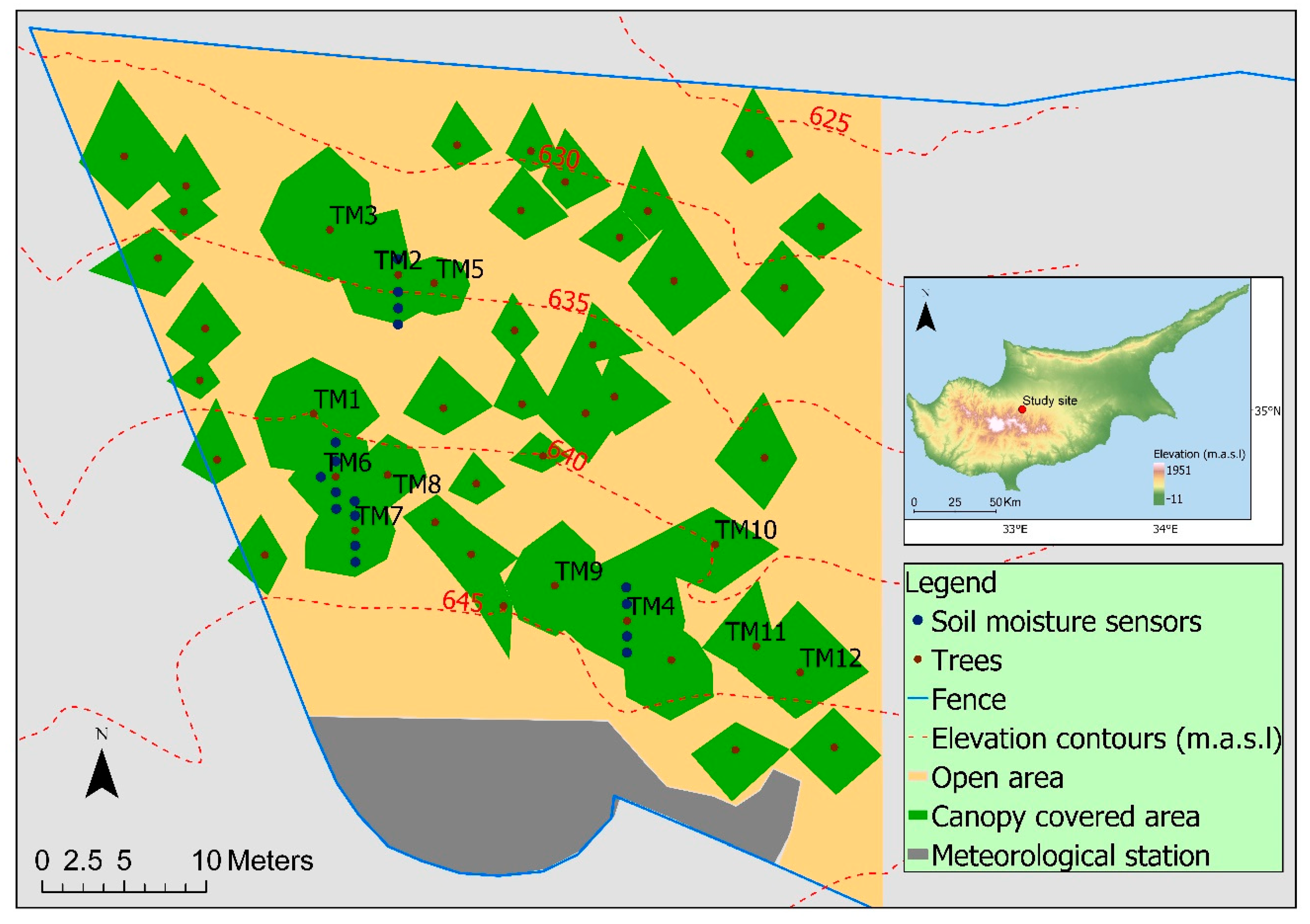
Our study was conducted from 29 December 2014, to 31 December 2017, within a fenced stand of P. brutia forest, on the northern foothills of the Troodos Mountains in Cyprus, at an elevation of ~620 meters above sea level (Figure 1). P. brutia formed a pure stand within the fenced area with a density of 200 trees per hectare. The site had a mean slope of 25 degrees and had a northern exposure. The soil was loamy with an average depth of 14 cm, and there were several spots with rock outcrops.
Meteorological data from an automatic meteorological station located in an open area within the study site were provided by the Department of Forests of Cyprus. Rainfall was measured with a tipping bucket rain gauge of 0.1 mm resolution, at a height of 1 m above ground surface. Air temperature and relative air humidity were measured at a height of 2 m. Solar radiation was measured by a pyranometer (W m−2), at a height of 2 m, and wind speed was measured with a three-cup anemometer at a height of 10 m.
2.2. Selection of Trees for Sap Flow Measurements
Eight trees were selected for monitoring, based on their diameter at breast height (DBH). The DBH represented the growing state of the trees and was able to be easily and accurately measured in field conditions [4]. We measured the circumference of 122 trees within the fenced area with a measuring tape, and computed the DBH of each tree by dividing its circumference with π. Similar to the method adopted by Reyes Acosta and Lubczynski [4], we calculated a histogram based on the trees’ DBH values, with 10 cm intervals, to guide the selection of the trees. We selected: (i) Two trees from the 10–20 cm DBH class, which made up 30% of the 122 trees in the stand; (ii) two trees from the 20–30 cm class, which made up 44% of the 122 trees; and (iii) four trees from the 30–40 cm DBH class, which made up 21% of the 122 trees in the stand. We selected a higher number of trees from the 30–40 cm DBH class, because the larger trees were expected to have higher azimuthal, radial, and between-tree variation in sap flow [11]. The DBH classes of 0–10 cm and >40 cm together represented less than 5% of the forest stand, so no trees from these two classes were selected for sap flow monitoring. The eight trees were located in the western part of the fenced area. These trees are referred to as TM1, TM2, TM3, TM4, TM5, TM6, TM7, and TM8 (Appendix A, Figure A1). The biometrics of the trees are presented in Table 1.
We measured the length of the longest branches in the eight cardinal and inter-cardinal directions for each selected tree, and also measured the length of the longest branches in the four cardinal directions for the remaining 37 trees in the western site of the fenced area. We used these data to estimate the canopy-projected areas of all 45 trees located in the western site of the fenced area using the triangulation method in ArcGIS®. Tree height was measured with an analogue height meter, and bark thickness was measured using a 5 cm-long bark gauge (Haglöf, Sweeden). The sapwood depth measurement is described in Section 2.3.
2.3. Relation between Sapwood and DBH
We measured the sapwood depth of 45 trees within the stand by taking tree core samples (at 1.6 m height) with an increment borer (Haglöf, Sweeden). The increment borer was 350 mm long and had a core diameter of 5.15 mm. The core samples were taken from the northwest to northeast site of the trunk, depending on the presence of cut stems or wounding. For the eight monitored trees, the core samples allowed for the measurement of sapwood depth at the diametrically opposite site of the sap flow sensor because of the considerable length of the increment borer (350 mm). We applied indicator dye (methyl orange and methyl blue) to the augured cores and determined the sapwood depth by the difference in colour between the sapwood and heartwood area on both sites, which is a method similar to previous studies [4,8,48,49,50]. Like Keyimu et al. [34], we developed a power relation between the DBH and the sapwood area of the P. brutia trees. We used a log transform of the variables to test the statistical significance of a non-zero slope of the linear regression equation with a t-test. We also took core samples and measured the sapwood depth of the four azimuthal directions of three trees to evaluate the sapwood depth variability along the trunk’s perimeter (see Supplementary Material, Figure S1).
2.4. Sap Flow
We used four sap flow Heat Ratio Method (HRM) instruments [51] (ICT international, Armidale, Australia) to determine sap flux densities of the TM2, TM4, TM6, and TM7 trees for the period from 1 October 2015, to 31 December 2017. We installed four more HRM instruments to monitor the sap flux densities of trees TM1, TM3, TM5, and TM8, from 20 October 2015, to 31 December 2017. Burgess et al. [51] referred to the HRM-measured variable as “sap velocity” (cm h−1)—however, following Fuchs et al. [49], Steppe et al. [52], and Vandegehuchte and Steppe [53], we have chosen to use the term, “sap flux density” (Jp) (cm3 cm−2 h−1). The sensors contained one heater and two temperature probes, positioned upstream and downstream of the heater. Each probe contained two thermistors that were positioned exactly at 7.5 and 22.5 mm from the tip of the measurement probes. These sensors, unlike the continuous heat methods that measure sap flow, were based on the fundamental heat conduction–convection equation presented by Marshall [54], and were further improved by Burgess et al. [51] in order to measure low and reverse flows. The temperature rise recorded by the probes, after the release of a pulse of heat, was converted to heat pulse velocity (Vh) and computed as follows:
where k is the thermal diffusivity of the fresh wood (cm2 s−1); x is the distance between the heater and the measurement needles (0.5 cm); and v1 and v2 are the differences between the initial temperature (°C) at the two thermocouples (downstream and upstream flow of the heater, respectively) and the temperature measured after a heat pulse was released. The thermal diffusivity k was computed after determining the thermal properties of sapwood, according to the procedures of Vandegehuchte and Steppe [53].
The installation procedure, computations, and corrections for natural thermal gradients, wound, and misalignment of the needles were conducted according to the method adopted by Burgess et al. [32,51] and Vandegehuchte et al. [55]. The probe misalignment was associated with the zero-flow adjustment which is crucial for the accuracy of the Jp measurements [51]. We used a drill guide to minimize probe misalignment. The direct determination of zero flows is usually done using destructive methods, such as by cutting the stem of the tree [7]. However, zero sap flow can alternatively be determined in periods when there is no biophysical driving force, during the night where vapor pressure deficit is at the lowest and during periods of substantial rainfall (soil moisture is at field capacity) [7,56]. We selected such periods of no biophysical driving force from the long-term data series to determine the zero flows (Supplementary Material, Figure S2). The Jp was then calculated according to the method by Burgess et al. [51] by using the Sap Flow Tool software [50], as follows:
where cs and cw refer to the specific heat capacities of sap (4182 J kg−1) [57] and wood (1200 J kg−1) [58], respectively, and ps is the sap density (1000 kg m−3); pb is the basic density of sapwood (kg m−3), and mc is the water content of sapwood (kg kg−1). We measured the volume and the fresh and oven-dried weight of augured sapwood samples for the computation of pb and mc (Supplementary Material, Table S2).
The HRM instruments have a resolution of 0.01 cm h−1 and an accuracy of 0.5 cm h−1, thus we discarded all observations between −0.5 and 0.5 cm h−1. The measurement interval of all HRM sensors was set to 1 h. All eight sensors were installed at breast height (1.3 m) facing north. We measured the wound width after the removal of the sensors and entered this into the correction algorithm in the Sap Flow Tool software [50]. Wounding was 0.20 cm in all trees. We reinstalled the sensors after observing noise in the data, which indicated increasing wound effects [50]. The dates of the sensor reinstallations are presented in the Supplementary Material, Table S3. For the conversion of Jp to sap flow, we defined the thermocouple positions as the midpoints of two concentric rings of the sapwood area (Ax) (0–15 and 15–30 mm sapwood depths). We multiplied the Jp by the sapwood area of each concentric ring. For trees with sapwood depth greater than 30 mm, we assumed that Jp declined linearly with sapwood depth, such that Jp became zero in the heartwood [59]. We conducted Heat Field Deformation (HFD) measurements at sapwood depths between 2 to 9 cm (8 observation points) to verify this assumption (see Section 2.5).
2.5. Radial Variability of Sap Flow
The radial variability of Jp was measured at 10 mm intervals between 20 and 90 mm with a Heat Field Deformation (HFD) sensor [60] (ICT international, Australia) at the northern side of TM1, between November 2015 and April 2016. Short-term HFD measurements on four other trees within the study area were conducted between March and April 2018. We refer to these trees as TM9 (DBH = 31.2 cm), TM10 (DBH = 33.7 cm), TM11 (DBH = 25.5 cm), and TM12 (DBH = 29.3 cm). The measurement interval of the HFD was 15 min. We used the average values of Jp of each tree at each depth interval to examine the relationship between sapwood depth and Jp. We tested the statistical significance of the regression slopes with a t-test.
2.6. Azimuthal Variability of Sap Flow
We measured the Jp with HRM sensors on both the northern and southern sides of TM6 and TM7 between January 2015 and August 2015. We selected these trees for long-term monitoring because they were neighboring, and thus would be able to give more information on the influential factors of the north and south variability. Also, these trees were of similar size and represented the DBH class with the highest number of trees (see Section 2.2). During July and August 2017, we measured Jp at the four azimuthal directions of the four big trees (see Section 3.4); TM1, TM2, TM3, and TM4. Hourly values with missing data were excluded from the computations. We tested the statistical significance of the difference between the north and any other azimuth with a t-test for serially-correlated data by adjusting the test statistic with the lag-1 autocorrelation [61]. The null hypothesis (Ho) was that the difference between the means of different azimuths would be zero, while the alternative hypothesis (Ha) was that the difference between the means would not be zero. The significance level was set to 5% (α = 0.05).
2.7. Soil Water Content
Eighteen soil moisture and temperature sensors (5TM, Decagon Devices, Pullman, WA, USA) were installed at 12 cm depth near TM2, TM4, TM6, and TM7 in November 2014 (Figure 1). We installed the sensors 1 and 2 m north and south of the tree stem, if soil was present, to capture the effects of shading and of the strong north–south slope. One sensor was installed 3 m south of TM2 and another sensor 1 m west of TM6. Yet another sensor was installed at 30 cm depth, 2 m north of tree TM7 where soil depth was greater than 24 cm. The accuracies of these sensors were ±3% of the volumetric water content and ±1 °C of the soil temperature. The sensors were connected to four Em50G wireless cellular data loggers (Decagon Devices, USA). The measurement interval for all soil moisture sensors was 1 h. A 2-factor variance analysis showed no statistically significant effect of the tree or the location of the sensor relative to the tree on the average soil moisture [46]. Therefore, we used the average soil moisture content (θ) of the 17 sensors at 12 cm depth for the analysis of soil moisture stress on transpiration. We used the average of two water potential sensors (Teros 21, Meter Group), placed at 12 cm soil depth, and the average volumetric soil moisture content of the 17 sensors to define the field capacity and wilting point. We used the common soil physical definition of −33 kPa for field capacity and −1500 kPa for wilting point. The observed average soil moisture content was 20% at field capacity (θfc) and 13% at wilting point (θwp). After 13% the change in soil moisture content was very slow and most likely dominated by evaporation through the thick mulch layer of pine needles. However, the trees did not wilt because they took up water from the fractured bedrock. We refer to soil moisture conditions below wilting point as soil moisture depletion.
2.8. Hydraulic Redistribution
The reverse flows (negative sap flow) measured by the sap flow sensors (see Section 2.4) were used as an indication of hydraulic redistribution. To further explore the occurrence of hydraulic redistribution, we installed two additional HRM sensors onto the roots of tree TM1—one at the east root and another at the west root, from 20 October 2015, to 3 July 2017. We examined hourly data where reverse sap flow occurred and compared them with meteorological parameters.
2.9. Daily and Nocturnal Transpiration
Transpiration (T) of each individual tree (mm) was computed by dividing sap flow by the corresponding ground area of the tree, estimated by Voronoi (Thiesen) polygons [46]. The average transpiration of all trees was computed as the area-weighted transpiration of the eight monitored trees. We identified and summed up total nocturnal sap flow (Qn) for all hours between the computed sunset and sunrise hours. Nocturnal sap flow is the result of two processes: stem refilling (Re) and nocturnal transpiration (Tn) [18,56,62]. Similarly to Fisher et al. [18], we applied the “forecasted refilling” method to separate the two processes. We assumed that stem filling would take place under declining sap flow and VPD only. For these conditions, the first two hourly nighttime sap flow observations were assumed to be stem-filling, and the slope (dT/dt) between these points was linearly extrapolated forward to zero. The area above the extrapolated line is identified as Tn and that below the curve is stem-refilling (Supplementary Material, Figure S3) [56]. We applied linear regressions between hourly sap flow at different sensors, in order to fill in any missing hourly data for the quantification of sap flow of all monitored trees.
3. Results and Discussion
3.1. Environmental Conditions
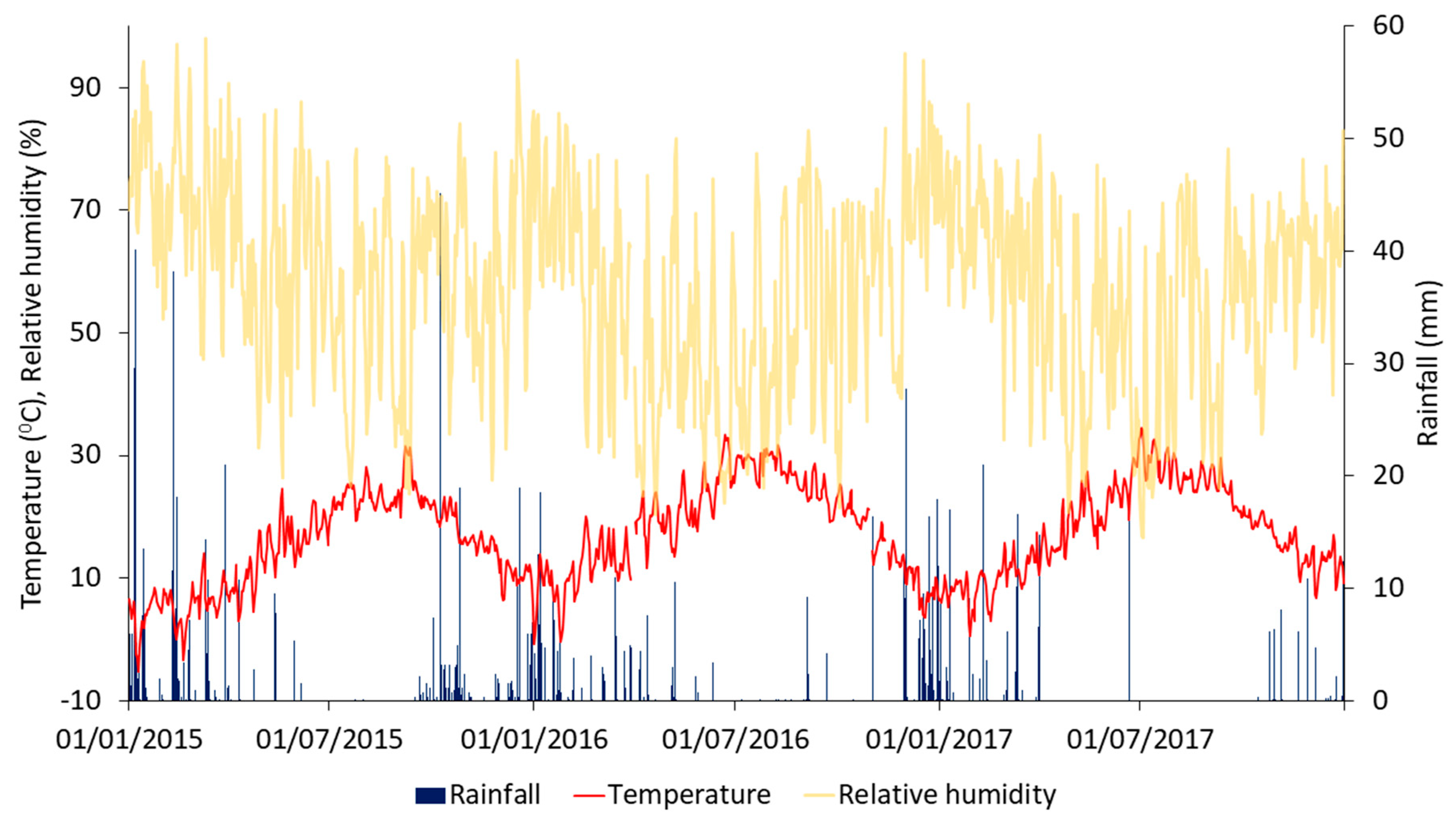
The daily rainfall (P), average daily temperature, and average daily relative humidity for the period between 1 January 2015, and 31 December 2017, is presented in Figure 2. Total rainfall was 507.2 mm in 2015, 358.8 mm in 2016, and 220.3 mm in 2017. The highest daily rainfall of 45.2 mm was recorded on 8 October 2015. The lowest average monthly minimum daily temperature was 3.9 °C in January 2015, and the highest average monthly maximum was 29.3 °C in July 2017. There were three days where the temperatures remained below zero (8–9 January 2015, and 19 February 2015). The lowest recorded absolute temperature was −7.7 °C on 9 January 2015, and the highest absolute temperature was 42.4 °C on 2 July 2017. The total reference evapotranspiration was 1277 mm in 2015, 1480 mm in 2016, and 1413 mm in 2017.
3.2. Sapwood Area and DBH
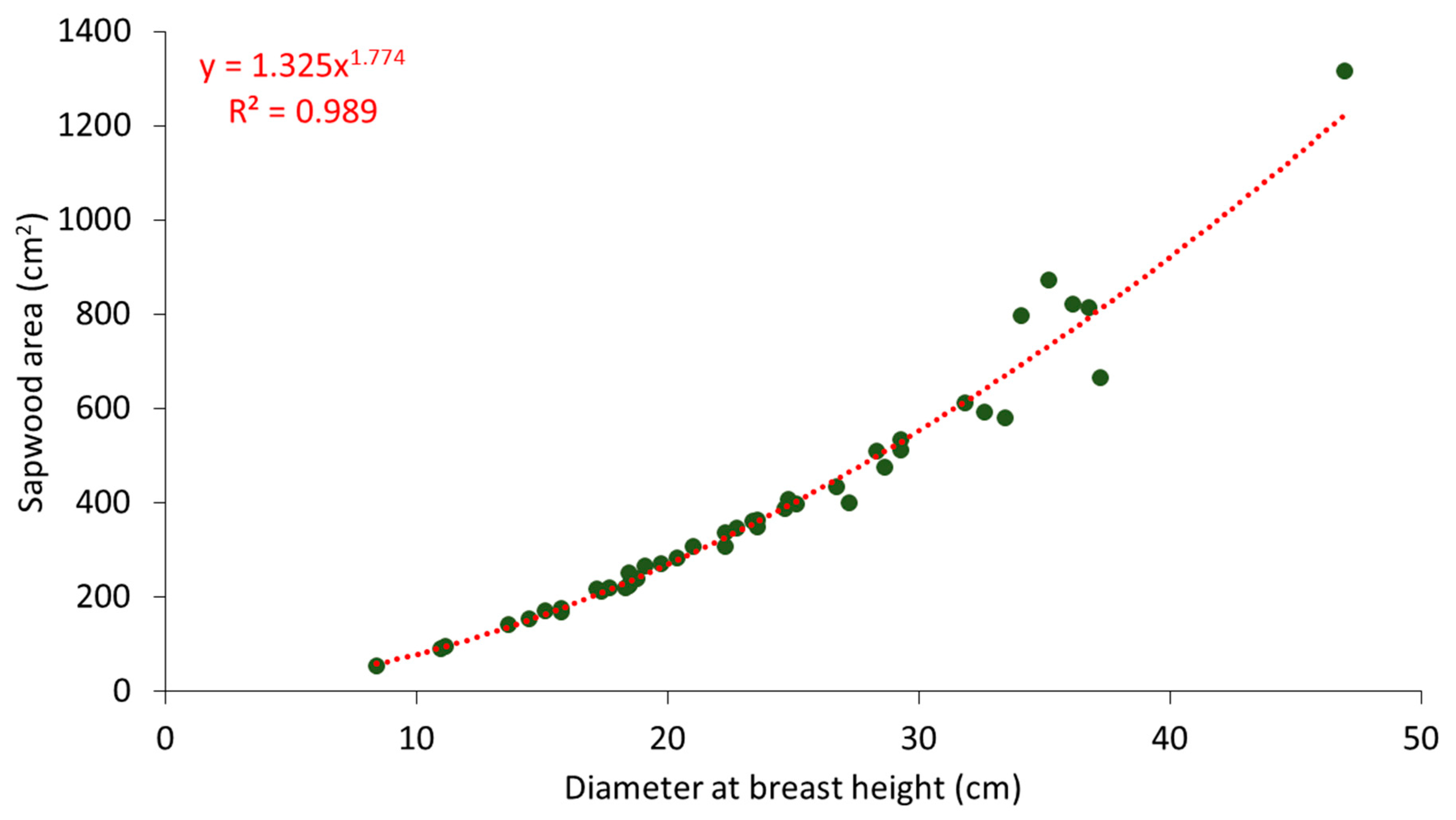
The relationship between sapwood area and DBH is presented in Figure 3. The sapwood area of the 45 P. brutia trees and the DBH values were well-fitted by a power function (Ax = 1.325 * DBH1.774, r2 = 0.989, p < 0.001). Observations showed very little difference in the depth of the sapwood cores taken from the four azimuthal directions of the trunk (Supplementary Material, Table S1). A similar power relation between sapwood area and DBH (Ax = 1.452 * DBH1.553) was found by Keyimu et al. [34], for Populus euphratica trees in an arid climate, at the lower reaches of the Tarim River in China. Our results show a larger increase in sapwood area with increasing DBH for P. brutia compared to the relations for Populus euphratica. Contrastingly, in a study about the relation between sapwood area and other tree parameters of the Mediterranean conifers Cedrus libani, Güney [63] found a linear relation between sapwood area and DBH.
3.3. Radial Variations of Sap Flux Density
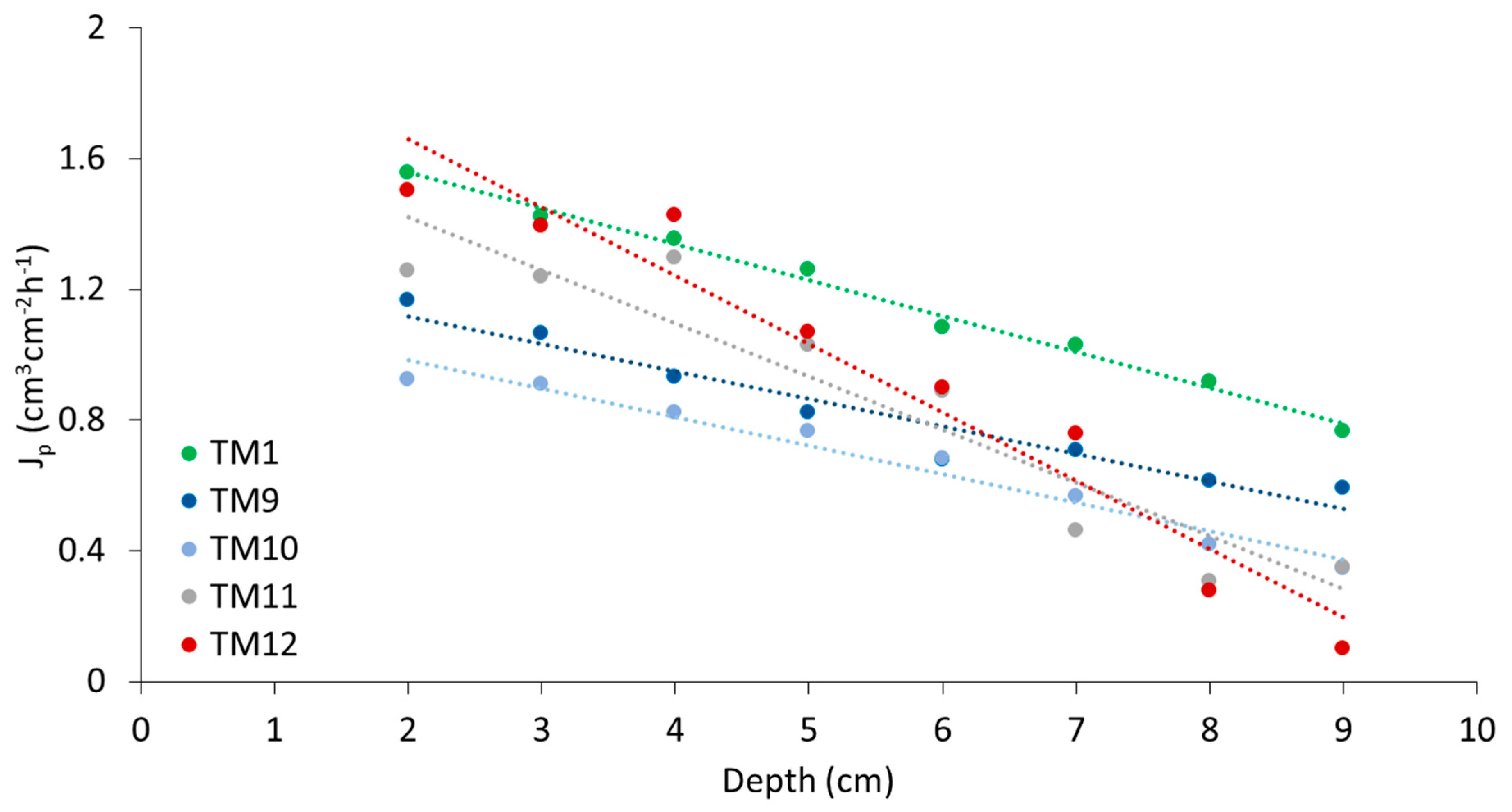
The 6-month HFD observations for TM1 show a linear decrease of the mean Jp with sapwood depth (r2 = 0.99, p < 0.001) (Figure 4). The mean Jp of the other four trees show similar linear relations (r2 = 0.89–0.97, p < 0.001). Small discrepancies were observed in TM11 and TM12, which had the highest Jp values at the 4 cm sapwood depth. The slightly steeper slopes of TM11 and TM12 could be expected because of their smaller DBHs (25 cm for TM11, 29 cm for TM12), relative to the 33 cm average DBH of the other three trees.
A near-linear decrease of Jp with sapwood depth was also observed in Pinus halepensis trees in Israel by Cohen et al. [6], while Liphschitz and Mendel [64] found that P. brutia and P. halepensis species had similar radial growth responses. According to Fuchs et al. [49], HFD is a valid tool for studying radial flux patterns, but for quantification of sap flow at low and medium Jp (<30 cm3 cm−2 h−1), highest accuracies are achieved with the HRM method. Other studies also reported higher sap flux accuracies with the HRM than with other sap flow methods [53,65].
3.4. Azimuthal Variations of Sap Flux Density
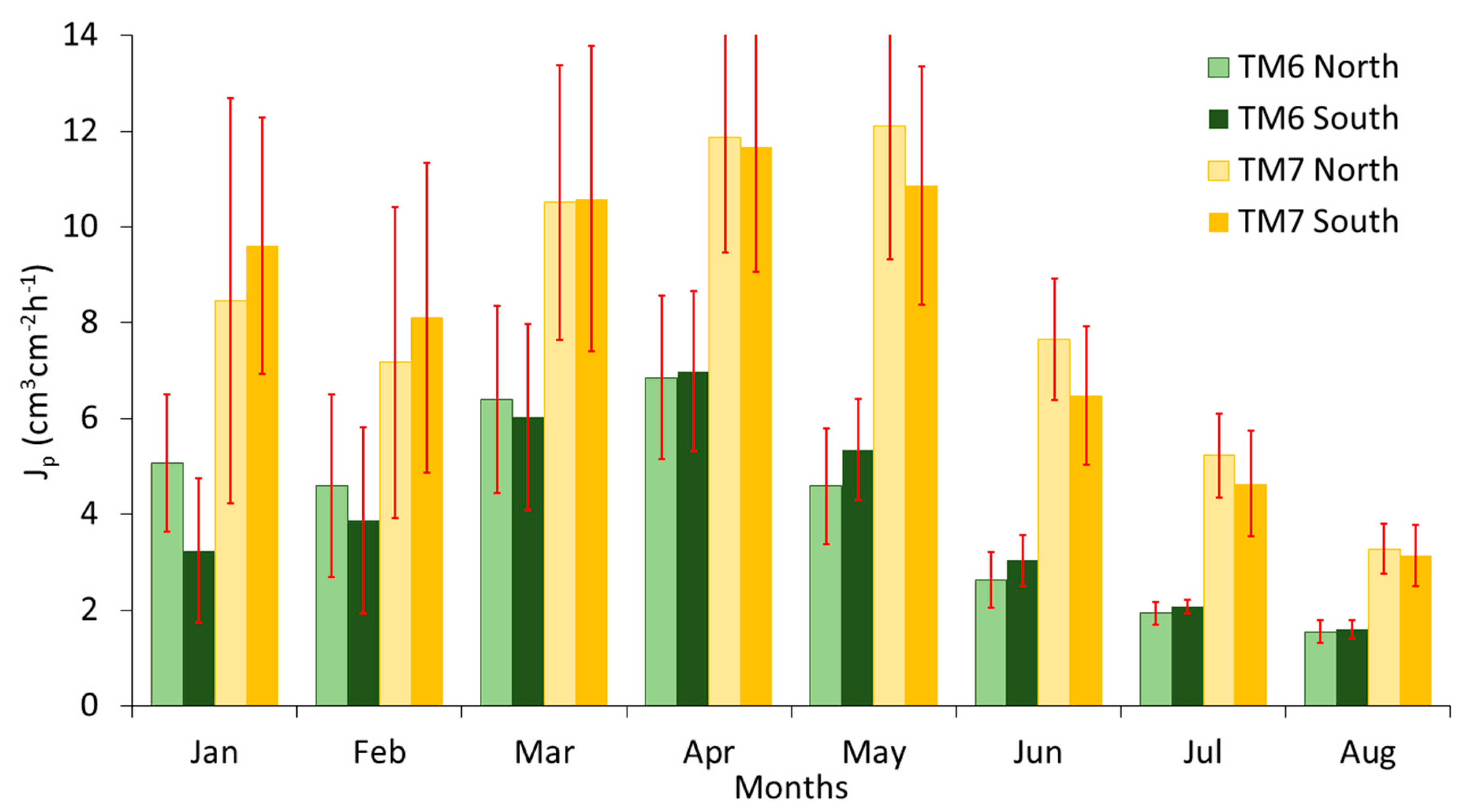
The monthly averages of the hourly Jp of the HRM sensors on the north (Jp-N) and south (Jp-S) of TM6 and TM7 trees are presented in Figure 5. The difference in sap flow between these two neighboring trees is most likely due to the much smaller open area and thus smaller soil moisture reservoir around TM6: 19.2 m2 versus 46.5 m2 for TM7 (Section 3.6), whereas their DBHs are nearly the same (Table 1). The differences between Jp-N and Jp-S are not constant over time and differ between trees. During the wet winter months, Jp-N is higher than Jp-S in TM7, while it is the opposite for TM6. In May, the situation reversed, with Jp-N lower than Jp-S in TM7, and Jp-N higher than Jp-S in TM6. The southern site of TM7 had a larger open area and deeper soils and, due to its location on the steep northern-facing slope (see Figure 1), was more exposed to solar radiation than any other azimuth of the TM6 and TM7 trees. However, the difference between the north and south Jp of both trees was not statistically significant (p = 0.57 for TM6, p = 0.18 for TM7). Seasonal changes in Jp at different azimuths have been found to be related to the seasonal variation in the proportion of the tree crown exposed to solar radiation [59]. In addition, Lu et al. [66], who applied localized irrigation treatments to mango trees, concluded that azimuthal variations could be the result of uneven distribution in soil moisture.
The Jp of the different azimuths for all trees are presented in Table 2. There was no pattern between the values of Jp and the different azimuths. Similar to our study, Cohen et al. [6] also found inconsistent relations between the Jp at different azimuths around the trunks of six forest species and three fruit trees in a Mediterranean climate. For all four trees (TM1–TM4) the Jp of the three azimuths were not significantly different from the Jp of the north-facing sensors, and the p-values were between 0.10 (TM2 Jp-N Jp-E) and 0.97 (TM4 Jp-N Jp-W), except for the east-facing sensor of the TM3 tree (p = 0.004). Even though the observations of this sensor were significantly different from the north facing sensor, the difference in the average sap flux density of the two sensors was just 5%. Moreover, comparing the average Jp-N with the average Jp of all four sensors, we found no significant differences (p = 0.430–0.880). The sap flux densities of our north-facing sensors were, on average, only 0.8% lower than the average sap flux densities of all four azimuth sensors. Thus, the Jp-N is used for all following results.
The coefficient of variation of the four azimuths ranged between 0.16 (TM3) and 0.28 (TM1). In their study about the spatial sap flow and xylem anatomical characteristics in olive trees (Spain), Lopez-Bernal et al. [67] reported higher azimuthal variability (CV = 0.54). Tseng et al. [15] also reported higher azimuthal variations (CV = 0.16–0.93) for Cryptomeria japonica trees in Taiwan.
3.5. Hydraulic Redistribution
The number of hourly reverse flow observations and the fractions of the reverse flows under different environmental conditions of the eight trees for the period between 20 October 2015, and 31 December 2017, are presented in Table 3. Reverse flows were, on average, less than 1% for both the total number of the total hourly sap flow observations and the total volumetric sap flow. The majority of the reverse flows occurred at night and during low VPD (Table 3). Total reverse flows ranged between −2 L (TM6) and −43 L (TM7) for the period between 20 October 2015, and 31 December 2017.
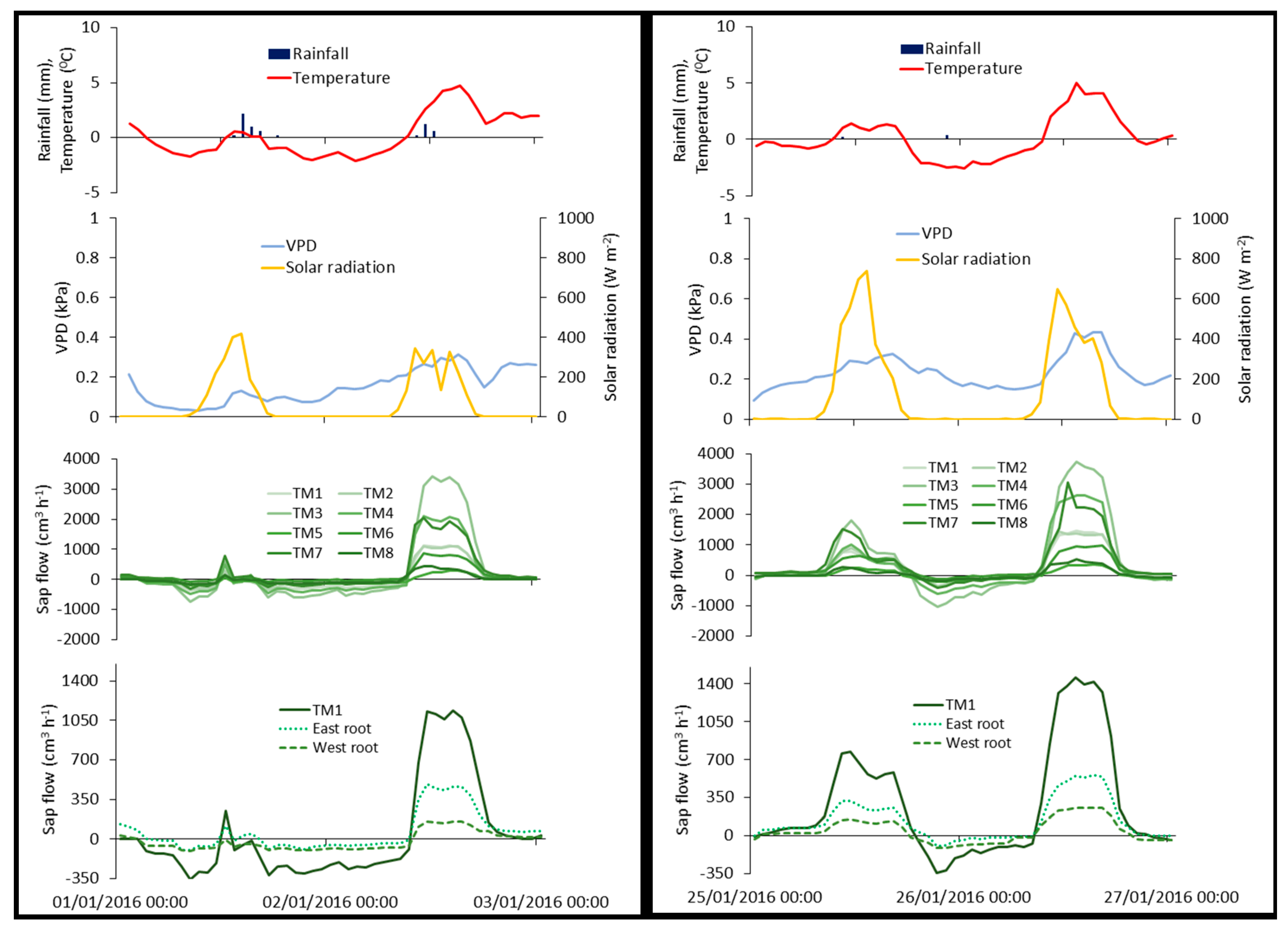
The lowest hourly absolute values of reverse flows for TM1 (−382.6 cm3 h−1), TM2 (−680.9 cm3 h−1), and TM3 (−1051.7 cm3 h−1) were observed on 27 January 2017, at 19:00 and ranged between −137.8 cm3 h−1 (TM8) and −1051.7 cm3 h−1 (TM3). The lowest hourly absolute values of reverse flows for TM4 (−465.2 cm3 h−1), TM6 (−317.1 cm3 h−1), and TM7 (−1420.1 cm3 h−1) were observed on 9 January 2015, at 04:00 (Figure 6). The lowest hourly observed value for TM5 (−215.8 cm3 h−1) and TM8 (−190.1 cm3 h−1) were observed on 25 January 2016, at 21:00. The absolute temperatures during these dates were −1.3 °C, −6.3 °C, and −2.3 °C, respectively. The results show that the highest absolute reverse flows occurred during negative temperatures without rainfall and with VPD higher than 0.1 kPa (Figure 6). Nadezhdina et al. [29] called this case of hydraulic redistribution, “frost-based reversal”. Their study on the sap flow of Douglas fir trees showed that reverse flows occurred during the night at below-zero temperatures. They concluded that this hydraulic redistribution mechanism may be a survival strategy of plants to avoid freezing. During the study period, reverse sap flow peaked at 8.9% of the maximum daily transpiration rates. Burgess et al. [68] reported a lower percentage (5–7%) in their study about the foliar uptake of the species Sequoia sempervirens. A higher percentage (25%) has been reported by Eller et al. [69] for the cloud forest species Drimys brasiliensis, though their study was conducted in a glasshouse. Finally, Li et al. [70] in their study on temperate continent-arid climates in China, reported that the reversal rates of sap flow of the species Tamarix ramosissima peaked at 10.7% of maximum transpiration rates.
Sap flow on the roots of TM1 (east and west) showed a similar pattern to the sap flow measured on the trunk of this tree (Figure 6). However, there were cases where reverse flows occurred only in one root, or only at the tree trunk. 13% of the 116 reverse flow observations for the TM1 trunk occurred without any reverse flow observations on the TM1 roots. However, 32% of the 121 reverse flow observations on the eastern root occurred without any reverse flow observations on the western root and tree trunk. Similarly, 23% of the 130 reverse flow observations on the western root occurred without any reverse flow observations on the eastern root and tree trunk. Of the total number of reverse flow observations for the TM1 trunk, 16% occurred at the same time as the reverse flow observations on the western root, 1% with reverse flow observations on the eastern root, and 70% with reverse flow observations on both roots. The lowest observed values for the trunk (−383 cm3 h−1) and for the east root (−164 cm3 h−1) were recorded on 27 January 2017. The lowest observed value for the west root (−113 cm3 h−1) was recorded on 25 January 2016 (Figure 6). Reverse flow was recorded on these days for the other trees too. The results indicated water movement from the trunk to the roots of the tree, and possibly the release of water to the soil. The occurrence of reverse flow observations in the roots could be an indication of the heterogeneous soil water conditions of the area [71].
3.6. Long-Term Daytime and Nocturnal Tree Transpiration
The linear relations between Jp of the north-facing sap flow sensors showed high correlations (r = 0.89–0.97) for the common period between 20 October 2015, and 31 December 2017, which justified the use of regression equations for filling in missing data. The total annual transpiration and percentages of nocturnal transpiration and stem refilling of the eight trees for the period between 1 January 2015, and 31 December 2017, is presented in Table 4. On average, stem refilling (Re) and nocturnal transpiration (Tn) were 3% and 15% of the total sap flow, respectively. Alvarado-Barrientos et al. [62] reported that the percentage of stem refilling to the total nocturnal sap flow for the species Quercus lancifolia, Alchornea latifolia, Alnus jorullensis, and Pinus pinula ranged between 21–25%, 6%, 5%, and 21–23%, respectively. A stem refilling percentage of 80% was reported by Yu et al. [56] for Populus euphratica trees in a hyper-arid environment in China.
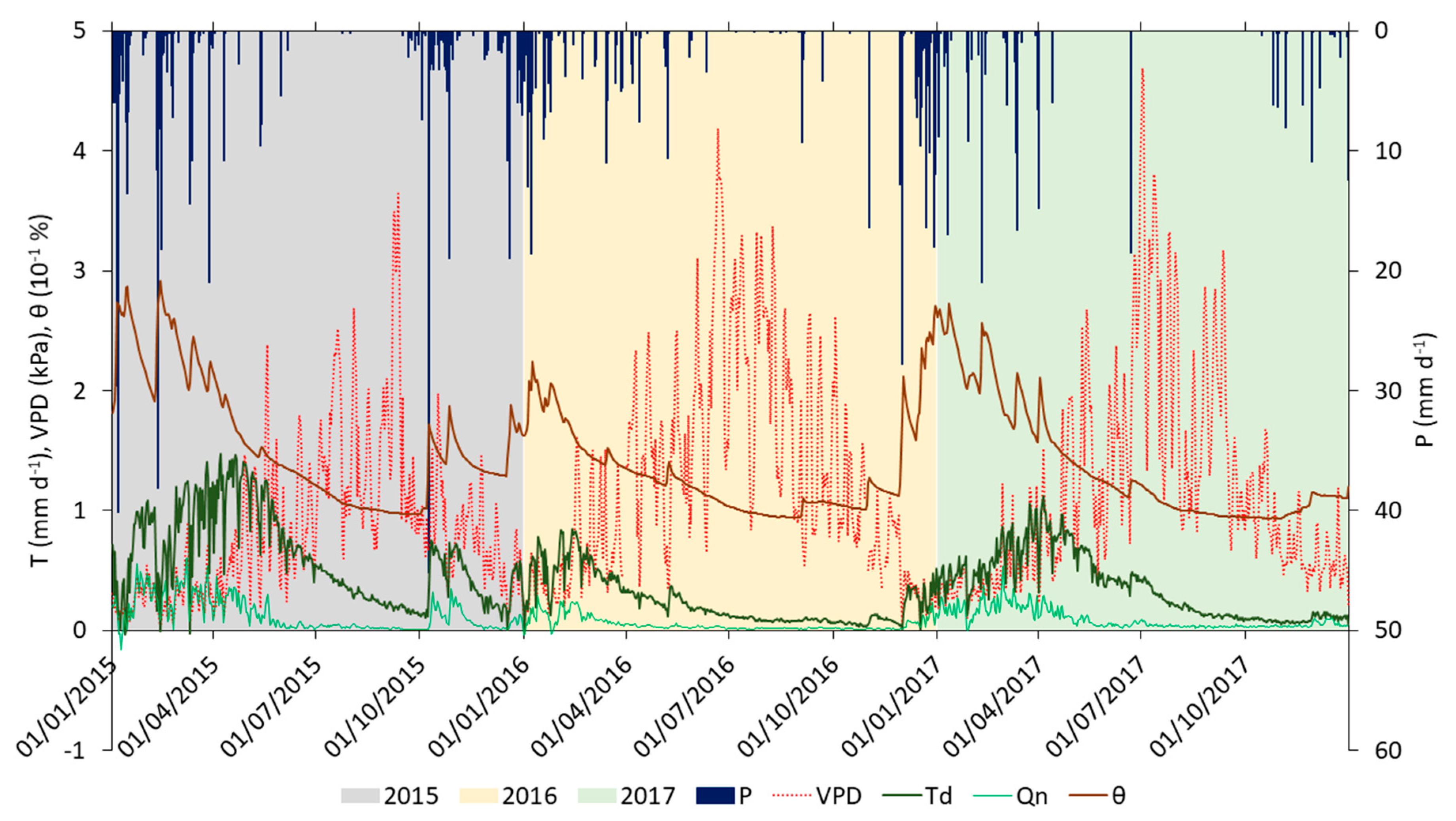
The vapor pressure deficit (VPD), daily rainfall (P), daytime transpiration (Td), nocturnal sap flow (Qn) and soil moisture (θ) for the years 2015, 2016, and 2017 are presented in Figure 7. The results show a seasonal pattern of transpiration. Even though rainfall was significantly lower in 2017 than in 2016, transpiration was higher (Table 5). This is due to the temporal distribution of rainfall and soil moisture during the year and the rain in the preceding fall months, which could recharge the fractured bedrock. Detailed water balance computations, based on throughfall, sap flow, and soil moisture observations, have shown that the trees at the site draw water from the bedrock fractures [46].
High levels of rain and soil moisture in January–March (winter) 2015 most likely recharged the bedrock fractures, resulting in high transpiration in April–June (spring) 2015. Transpiration reached the maximum record of 1.8 mm/d on 20 April. Between October and December (fall) 2015, we observed an intermediate period, where two high rainfall events—45.2 mm on 8 October 2015, and 19 mm on 26 October 2015, provided sufficient levels of soil moisture, leading to high transpiration rates. Even though we had high rainfall during this period, soil moisture did not exceed field capacity. A decrease in soil moisture and transpiration was observed. During winter 2016, soil moisture and transpiration were much lower than in winter 2015. The lowest observed T/P ratio was 0.10 in fall 2016. This period was characterized by a large number of days below wilting point at the beginning (60 days). However, during the last 15 days of the year, significant rainfall events (88 mm) kept soil moisture above field capacity. Rain in winter 2017 was the lowest in all three years. However, transpiration during the cool January–February months was fairly similar for all three years: 50.3 mm (2015), 41.4 m (2016), and 39.1 mm (2017). Differences became more pronounced in March, where transpiration showed the same pattern as the average soil moisture: 41.5 mm and 22% in 2015, 15.8 mm and 14% in 2016, and 29.4 mm and 18% in 2017. More days exceeded the field capacity in winter 2017 than in winter 2016, and we observed higher levels of transpiration in spring and summer 2017 than during those seasons in 2016.
Nocturnal sap flow (Qn) occurred during the wet season when soil moisture was above the θwp, while during the dry season, nocturnal transpiration was close or equal to zero (Figure 7). Total nocturnal sap flow (Qn) in our study was, on average, 18% of the total transpiration. Nocturnal sap flow has been found among many species and climatic regions across the world [17]. In his review paper, Forster [17] estimated that nocturnal sap flow for the Mediterranean regions was about 11% of the daily sap flow. However, in contrast to our study, they found that higher levels of nocturnal sap flow occurred during the dry period than the wet period. Liu et al. [72] reported similar seasonality of nocturnal sap flow as found in our study. According to these authors, the reason for this seasonality is because the nighttime period during spring and autumn is longer than in summer, meaning there is more time for nocturnal sap flow to accumulate.
The seasonality of transpiration we found in our study is typical for most Mediterranean tree species [23,24]. The average annual transpiration in our study site for the three-year period was 180 mm. Yaseef et al. [73] found an average annual transpiration of 129 mm for eight trees during a four-year period (2003–2007) in a Pinus halepensis forest in Israel, which was a semi-arid Mediterranean environment (average annual rainfall 285 mm). Brito et al. [74] measured the sap flow of 10 trees in a Pinus canariensis forest from March–September, and found there was a total transpiration of 60 mm in 2008 (annual rainfall 369 mm) and 140 mm in 2009 (annual rainfall 275 mm). For the same period, we found transpiration rates of 172 mm in 2015, 49 mm in 2016, and 114 mm in 2017. According to Brito et al. [74], Pinus canariensis are able to survive and grow in the semi-arid Canary islands due to their ability to tap water accumulated from rainfall in the cold and wet seasons from the deeper soil layers, which covers their transpiration needs during the dry summer period [74,75]. Thus, they concluded that the effect of drought on tree water status was primarily related to wet season precipitation, rather than to the dry summers. In our case, rainfall during the period of November–April was 41% lower in 2016 (219.4) than in 2015 (371.4 mm). The bedrock water was probably completely depleted in October 2016, as the transpiration rates measured then were almost zero.
4. Conclusions
In this study, we examined the Jp of eight P. brutia trees in various environmental conditions. The radial measurements of sap flux densities showed a linear decrease with sapwood depth. We found that the differences between sap flux density measurements at different azimuths differed between trees and with time. For only one of the 12 azimuthal pairs of observations the sap flow at the north-facing sensor was significantly different from the sap flow at the non-north-facing sensor (p = 0.004). However, the sap flow at the north-facing sensor was just 5% lower than that at the non-north-facing sensor. The sap flux density at the north-facing sensors was, on average, only 0.8% lower than the average sap flux densities of all four azimuths.
We discovered that P. brutia trees hydraulically redistributed water under specific meteorological conditions. We observed reverse flows in both the stems and the roots during low VPD and rainfall, which is an indication that water was transferred from the tree to the roots and eventually to the soil layer, a process referred to as “foliar water uptake”. Reverse flows were also observed during negative temperatures in the absence of rainfall, indicating that P. brutia trees have a frost-avoidant mechanism.
The transpiration of P. brutia varied from year to year, as they rely both on the amount and temporal distribution of rainfall. The number of days with soil moisture above field capacity during the winter leads to higher levels of transpiration during the months in spring, due to bedrock water recharge. Low transpiration levels indicate that relatively more water is lost to evaporation over the dry years. There are prolonged periods of soil moisture depletion where P. brutia rely on bedrock water for their transpiration needs. There was an immediate increase of P. brutia sap flow after rainfall events. Nocturnal tree transpiration made a significant contribution (15%) to the overall transpiration and occurred during the wet period when soil moisture was above wilting point.
Further research is needed to improve our understanding of the multi-year transpiration and growth dynamics of P. brutia, and their responses and water uptake during prolonged periods of drought.
Supplementary Materials
The following are available online at https://www.mdpi.com/2073-4441/10/8/1039/s1.
Author Contributions
M.E. and A.B.: study design, data collection, analysis and interpretation of data and paper writing. H.D.: data collection and contribution to the paper writing. M.W.L.: interpretation of data and contribution to the paper writing. All authors have revised and approved the final manuscript.
Funding
This research has received funding from the European Union’s Horizon 2020 Research and Innovation programme, under Grant Agreement 641,739 (BINGO Project).
Acknowledgments
We would like to express our sincere thanks to Andreas Christou, Konstantinos Rovanias and Aristarchos Aristarchou from the Cyprus Department of Forests and to Filippos Tymvios and Demetris Charalambous from the Cyprus Department of Meteorology for their support on this research. We would like to thank also Elias Giannakis, Christos Zoumides and Corrado Camera for their valuable help during field work. We are very grateful to the four reviewers, who helped us correct and improve our analysis and explanations.
Conflicts of Interest
The authors declare no conflict of interest.
Appendix A
Figure A1.
Heat ratio method (HRM) sap flow sensors installed on P. brutia trees TM2, TM3, TM4, and TM5; trees and heat field deformation (HFD) sap flow sensor on tree TM11.
Figure A1.
Heat ratio method (HRM) sap flow sensors installed on P. brutia trees TM2, TM3, TM4, and TM5; trees and heat field deformation (HFD) sap flow sensor on tree TM11.

References
- IPCC Summary for Policymakers. In Climate Change 2014: Impacts, Adaptation, and Vulnerability. Part A: Global and Sectoral Aspects. Contribution of Working Group II to the Fifth Assessment Report of the Intergovernmental Panel on Climate Change; Field, C.B.; Barros, V.R.; Dokken, D.J.; Mach, K.J.; Mastrandrea, M.D.; Bilir, T.E.; Chatterjee, M.; Ebi, K.L.; Estrada, Y.O.; Genova, R.C.; et al. (Eds.) Cambridge University Press: Cambridge, UK; New York, NY, USA, 2014; pp. 1–32. [Google Scholar]
- Steppe, K.; Vandegehuchte, M.W.; Tognetti, R.; Mencuccini, M. Sap flow as a key trait in the understanding of plant hydraulic functioning. Tree Physiol. 2015, 35, 341–345. [Google Scholar] [CrossRef] [PubMed] [Green Version]
- Chang, X.; Zhao, W.; He, Z. Radial pattern of sap flow and response to microclimate and soil moisture in Qinghai spruce (Picea crassifolia) in the upper Heihe River Basin of arid northwestern China. Agric. For. Meteorol. 2014, 187, 14–21. [Google Scholar] [CrossRef]
- Reyes-Acosta, J.L.; Lubczynski, M.W. Optimization of dry-season sap flow measurements in an oak semi-arid open woodland in Spain. Ecohydrology 2014, 7, 258–277. [Google Scholar] [CrossRef]
- Rabbel, I.; Bogena, H.; Neuwirth, B.; Diekkrüger, B. Using Sap Flow Data to Parameterize the Feddes Water Stress Model for Norway Spruce. Water 2018, 10, 279. [Google Scholar] [CrossRef]
- Cohen, Y.; Cohen, S.; Cantuarias-Aviles, T.; Schiller, G. Variations in the radial gradient of sap velocity in trunks of forest and fruit trees. Plant Soil 2008, 305, 49–59. [Google Scholar] [CrossRef]
- Forster, M. How Reliable Are Heat Pulse Velocity Methods for Estimating Tree Transpiration? Forests 2017, 8, 350. [Google Scholar] [CrossRef]
- Schwärzel, K.; Zhang, L.; Strecker, A.; Podlasly, C. Improved Water Consumption Estimates of Black Locust Plantations in China’s Loess Plateau. Forests 2018, 9, 201. [Google Scholar] [CrossRef]
- Jaskierniak, D.; Benyon, R.; Kuczera, G.; Robinson, A. A new method for measuring stand sapwood area in forests. Ecohydrology 2015, 8, 504–517. [Google Scholar] [CrossRef]
- David, T.S.; Pinto, C.A.; Nadezhdina, N.; Kurz-Besson, C.; Henriques, M.O.; Quilhó, T.; Cermak, J.; Chaves, M.M.; Pereira, J.S.; David, J.S. Root functioning, tree water use and hydraulic redistribution in Quercus suber trees: A modeling approach based on root sap flow. For. Ecol. Manag. 2013, 307, 136–146. [Google Scholar] [CrossRef]
- Delzon, S.; Sartore, M.; Granier, A.; Loustau, D. Radial profiles of sap flow with increasing tree size in maritime pine. Tree Physiol. 2004, 24, 1285–1293. [Google Scholar] [CrossRef] [PubMed] [Green Version]
- Nadezhdina, N.; Cermak, J.; Ceulemans, R. Radial patterns of sap flow in woody stems of dominant and understory species: Scaling errors associated with positioning of sensors. Tree Physiol. 2002, 22, 907–918. [Google Scholar] [CrossRef] [PubMed]
- Ford, C.R.; McGuire, M.A.; Mitchell, R.J.; Teskey, R.O. Assessing variation in the radial profile of sap flux density in Pinus species and its effect on daily water use. Tree Physiol. 2004, 24, 241–249. [Google Scholar] [CrossRef] [PubMed] [Green Version]
- Loustau, D.; Domec, J.-C.; Bosc, A. Interpreting the variations in xylem sap flux density within the trunk of maritime pine (Pinus pinaster Ait.): Application of a model for calculating water flows at tree and stand levels. Ann. des Sci. For. 1998, 55, 29–46. [Google Scholar] [CrossRef]
- Tseng, H.; Chiu, C.-W.; Laplace, S.; Kume, T. Can we assume insignificant temporal changes in spatial variations of sap flux for year-round individual tree transpiration estimates? A case study on Cryptomeria japonica in central Taiwan. Trees 2017, 31, 1239–1251. [Google Scholar] [CrossRef]
- Shinohara, Y.; Tsuruta, K.; Ogura, A.; Noto, F.; Komatsu, H.; Otsuki, K.; Maruyama, T. Azimuthal and radial variations in sap flux density and effects on stand-scale transpiration estimates in a Japanese cedar forest. Tree Physiol. 2013, 33, 550–558. [Google Scholar] [CrossRef] [PubMed] [Green Version]
- Forster, M.A. How significant is nocturnal sap flow? Tree Physiol. 2014, 34, 757–765. [Google Scholar] [CrossRef] [PubMed] [Green Version]
- Fisher, J.B.; Baldocchi, D.D.; Misson, L.; Dawson, T.E.; Goldstein, A.H. What the towers don’t see at night: Nocturnal sap flow in trees and shrubs at two AmeriFlux sites in California. Tree Physiol. 2007, 27, 597–610. [Google Scholar] [CrossRef] [PubMed]
- Klein, T.; Cohen, S.; Paudel, I.; Preisler, Y.; Rotenberg, E.; Yakir, D. Diurnal dynamics of water transport, storage and hydraulic conductivity in pine trees under seasonal drought. IForest 2016, 9, 710. [Google Scholar] [CrossRef]
- Zhao, C.Y.; Si, J.H.; Feng, Q.; Yu, T.F.; Li, P. Du Comparative study of daytime and nighttime sap flow of Populus euphratica. Plant Growth Regul. 2017, 82, 353–362. [Google Scholar] [CrossRef]
- Buckley, T.N.; Turnbull, T.L.; Pfautsch, S.; Adams, M.A. Nocturnal water loss in mature subalpine Eucalyptus delegatensis tall open forests and adjacent E. pauciflora woodlands. Ecol. Evol. 2011, 1, 435–450. [Google Scholar] [CrossRef] [PubMed]
- Fuentes, S.; Mahadevan, M.; Bonada, M.; Skewes, M.A.; Cox, J.W. Night-time sap flow is parabolically linked to midday water potential for field-grown almond trees. Irrig. Sci. 2013, 31, 1265–1276. [Google Scholar] [CrossRef]
- Forner, A.; Aranda, I.; Granier, A.; Valladares, F. Differential impact of the most extreme drought event over the last half century on growth and sap flow in two coexisting Mediterranean trees. Plant Ecol. 2014, 215, 703–719. [Google Scholar] [CrossRef] [Green Version]
- Chirino, E.; Bellot, J.; Sánchez, J.R. Daily sap flow rate as an indicator of drought avoidance mechanisms in five Mediterranean perennial species in semi-arid southeastern Spain. Trees 2011, 25, 593–606. [Google Scholar] [CrossRef]
- Crosbie, R.S.; Wilson, B.; Hughes, J.D.; McCulloch, C. The upscaling of transpiration from individual trees to areal transpiration in tree belts. Plant Soil 2007, 297, 223–232. [Google Scholar] [CrossRef]
- David, T.S.; Ferreira, M.I.; Cohen, S.; Pereira, J.S.; David, J.S. Constraints on transpiration from an evergreen oak tree in southern Portugal. Agric. For. Meteorol. 2004, 122, 193–205. [Google Scholar] [CrossRef]
- Paço, T.A.; David, T.S.; Henriques, M.O.; Pereira, J.S.; Valente, F.; Banza, J.; Pereira, F.L.; Pinto, C.; David, J.S. Evapotranspiration from a Mediterranean evergreen oak savannah: The role of trees and pasture. J. Hydrol. 2009, 369, 98–106. [Google Scholar] [CrossRef]
- David, T.S.; Henriques, M.O.; Kurz-Besson, C.; Nunes, J.; Valente, F.; Vaz, M.; Pereira, J.S.; Siegwolf, R.; Chaves, M.M.; Gazarini, L.C.; et al. Water-use strategies in two co-occurring Mediterranean evergreen oaks: Surviving the summer drought. Tree Physiol. 2007, 27, 793–803. [Google Scholar] [CrossRef] [PubMed]
- Nadezhdina, N.; David, T.S.; David, J.S.; Ferreira, M.I.; Dohnal, M.; Tesař, M.; Gartner, K.; Leitgeb, E.; Nadezhdin, V.; Cermak, J.; et al. Trees never rest: The multiple facets of hydraulic redistribution. Ecohydrology 2010, 3, 431–444. [Google Scholar] [CrossRef]
- Prieto, I.; Armas, C.; Pugnaire, F.I. Water release through plant roots: New insights into its consequences at the plant and ecosystem level. New Phytol. 2012, 193, 830–841. [Google Scholar] [CrossRef] [PubMed]
- Richards, J.H.; Caldwell, M.M. Hydraulic lift: Substantial nocturnal water transport between soil layers by Artemisia tridentata roots. Oecologia 1987, 73, 486–489. [Google Scholar] [CrossRef] [PubMed]
- Burgess, S.S.O.; Turner, N.C.; Ong, C.K. The redistribution of soil water by tree root systems. Oecologia 1998, 115, 306–311. [Google Scholar] [CrossRef] [PubMed]
- Ellison, D.; Morris, C.E.; Locatelli, B.; Sheil, D.; Cohen, J.; Murdiyarso, D.; Gutierrez, V.; van Noordwijk, M.; Creed, I.F.; Pokorny, J.; et al. Trees, forests and water: Cool insights for a hot world. Glob. Environ. Chang. 2017, 43, 51–61. [Google Scholar] [CrossRef] [Green Version]
- Keyimu, M.; Halik, Ü.; Rouzi, A. Relating Water Use to Tree Vitality of Populus euphratica Oliv. in the Lower Tarim River, NW China. Water 2017, 9, 622. [Google Scholar] [CrossRef]
- Gu, D.; Wang, Q.; Otieno, D. Canopy Transpiration and Stomatal Responses to Prolonged Drought by a Dominant Desert Species in Central Asia. Water 2017, 9, 404. [Google Scholar] [CrossRef]
- Zeppel, M.; Macinnis-Ng, C.M.O.; Ford, C.R.; Eamus, D. The response of sap flow to pulses of rain in a temperate Australian woodland. Plant Soil 2008, 305, 121–130. [Google Scholar] [CrossRef] [Green Version]
- Zhao, W.; Liu, B. The response of sap flow in shrubs to rainfall pulses in the desert region of China. Agric. For. Meteorol. 2010, 150, 1297–1306. [Google Scholar] [CrossRef]
- Klein, T.; Rotenberg, E.; Cohen-Hilaleh, E.; Raz-Yaseef, N.; Tatarinov, F.; Preisler, Y.; Ogée, J.; Cohen, S.; Yakir, D. Quantifying transpirable soil water and its relations to tree water use dynamics in a water-limited pine forest. Ecohydrology 2014, 7, 409–419. [Google Scholar] [CrossRef]
- Small, E.E.; McConnell, J.R. Comparison of soil moisture and meteorological controls on pine and spruce transpiration. Ecohydrology 2008, 1, 205–214. [Google Scholar] [CrossRef]
- Schwinning, S. The ecohydrology of roots in rocks. Ecohydrology 2010, 3, 238–245. [Google Scholar] [CrossRef]
- Barbeta, A.; Mejía-Chang, M.; Ogaya, R.; Voltas, J.; Dawson, T.E.; Peñuelas, J. The combined effects of a long-term experimental drought and an extreme drought on the use of plant-water sources in a Mediterranean forest. Glob. Chang. Biol. 2015, 21, 1213–1225. [Google Scholar] [CrossRef] [PubMed]
- Chambel, M.R.; Climent, J.; Pichot, C.; Ducci, F. Mediterranean Pines (Pinus halepensis Mill. and brutia Ten.). In Forest Tree Breeding in Europe: Current State-of-the-Art and Perspectives; Pâques, L.E., Ed.; Springer: Dordrecht, The Netherlands, 2013; pp. 229–265. [Google Scholar]
- Boydak, M. Silvicultural characteristics and natural regeneration of Pinus brutia Ten.—A review. Plant Ecol. 2004, 171, 153–163. [Google Scholar] [CrossRef]
- Nahal, I. Le Pin brutia (Pinus brutia Ten. subsp. brutia). For. Mediterr. 1983, 5, 165–172. [Google Scholar]
- Polade, S.D.; Gershunov, A.; Cayan, D.R.; Dettinger, M.D.; Pierce, D.W. Precipitation in a warming world: Assessing projected hydro-climate changes in California and other Mediterranean climate regions. Sci. Rep. 2017, 7, 10783. [Google Scholar] [CrossRef] [PubMed]
- Eliades, M.; Bruggeman, A.; Lubczynski, M.W.; Christou, A.; Camera, C.; Djuma, H. The water balance components of Mediterranean pine trees on a steep mountain slope during two hydrologically contrasting years. J. Hydrol. 2018, 562, 712–724. [Google Scholar] [CrossRef]
- Camera, C.; Bruggeman, A.; Hadjinicolaou, P.; Pashiardis, S.; Lange, M.A. Evaluation of interpolation techniques for the creation of gridded daily precipitation (1 × 1 km2); Cyprus, 1980–2010. J. Geophys. Res. Atmos. 2014, 119, 693–712. [Google Scholar] [CrossRef]
- Fan, J.; Guyot, A.; Ostergaard, K.T.; Lockington, D.A. Effects of earlywood and latewood on sap flux density-based transpiration estimates in conifers. Agric. For. Meteorol. 2018, 249, 264–274. [Google Scholar] [CrossRef]
- Fuchs, S.; Leuschner, C.; Link, R.; Coners, H.; Schuldt, B. Calibration and comparison of thermal dissipation, heat ratio and heat field deformation sap flow probes for diffuse-porous trees. Agric. For. Meteorol. 2017, 244–245, 151–161. [Google Scholar] [CrossRef]
- Burgess, S.S.O.; Downey, A. SFM1 Sapflow Meter Manual; ICT International Pty Ltd.: Armidale, NSW, Australia, 2014. [Google Scholar]
- Burgess, S.S.; Adams, M.A.; Turner, N.C.; Beverly, C.R.; Ong, C.K.; Khan, A.A.; Bleby, T.M. An improved heat pulse method to measure low and reverse rates of sap flow in woody plants. Tree Physiol. 2001, 21, 589–598. [Google Scholar] [CrossRef] [PubMed] [Green Version]
- Steppe, K.; De Pauw, D.J.W.; Doody, T.M.; Teskey, R.O. A comparison of sap flux density using thermal dissipation, heat pulse velocity and heat field deformation methods. Agric. For. Meteorol. 2010, 150, 1046–1056. [Google Scholar] [CrossRef]
- Vandegehuchte, M.W.; Steppe, K. Sap-flux density measurement methods: Working principles and applicability. Funct. Plant Biol. 2013, 40, 213–223. [Google Scholar] [CrossRef]
- Marshall, D.C. Measurement of Sap Flow in Conifers by Heat Transport. Plant Physiol. 1958, 33, 385–396. [Google Scholar] [CrossRef] [PubMed]
- Vandegehuchte, M.W.; Burgess, S.S.O.; Downey, A.; Steppe, K. Influence of stem temperature changes on heat pulse sap flux density measurements. Tree Physiol. 2015, 35, 346–353. [Google Scholar] [CrossRef] [PubMed]
- Yu, T.; Feng, Q.; Si, J.; Mitchell, P.J.; Forster, M.A.; Zhang, X.; Zhao, C. Depressed hydraulic redistribution of roots more by stem refilling than by nocturnal transpiration for Populus euphratica Oliv. in situ measurement. Ecol. Evol. 2018, 8, 2607–2616. [Google Scholar] [CrossRef] [PubMed]
- Lide, D.R. CRC Handbook of Chemistry and Physics: A Ready-Reference Book of Chemical and Phyical Data, 73rd ed.; CRC Press: Boca Raton, FL, USA, 1990. [Google Scholar]
- Becker, P.; Edwards, W.R.N. Corrected heat capacity of wood for sap flow calculations. Tree Physiol. 1999, 19, 767–768. [Google Scholar] [CrossRef] [PubMed]
- Looker, N.; Martin, J.; Jencso, K.; Hu, J. Contribution of sapwood traits to uncertainty in conifer sap flow as estimated with the heat-ratio method. Agric. For. Meteorol. 2016, 223, 60–71. [Google Scholar] [CrossRef] [Green Version]
- Nadezhdina, N.; Cermak, J.; Nadezhdin, V. Heat field deformation method for sap flow measurements. In 4th International Workshop “Measuring Sap Flow in Intact Plants”; IUFRO Publications: Brno, Czech Republic; Publishing House of Mendel University: Zidlochovice, Czech Republic, 1998; pp. 72–92. [Google Scholar]
- Wilks, D.S. Statistical Methods in the Atmospheric Sciences; Academic Press: Cambridge, MA, USA, 2006. [Google Scholar]
- Alvarado-Barrientos, M.S.; Holwerda, F.; Geissert, D.R.; Muñoz-Villers, L.E.; Gotsch, S.G.; Asbjornsen, H.; Dawson, T.E. Nighttime transpiration in a seasonally dry tropical montane cloud forest environment. Trees 2015, 29, 259–274. [Google Scholar] [CrossRef]
- Güney, A.; Küppers, M.; Rathgeber, C.; Şahin, M.; Zimmermann, R. Intra-annual stem growth dynamics of Lebanon Cedar along climatic gradients. Trees 2017, 31, 587–606. [Google Scholar] [CrossRef]
- Liphschitz, N.; Mendel, Z. Comparative radial growth of Pinus halepensis Mill. and Pinus brutia in Israel. For. Mediterr. 1987, 9, 115–117. [Google Scholar]
- Bleby, T.M.; Burgess, S.S.O.; Adams, M.A. A validation, comparison and error analysis of two heat-pulse methods for measuring sap flow in Eucalyptus marginata saplings. Funct. Plant Biol. 2004, 31, 645. [Google Scholar] [CrossRef]
- Lu, P.; Muller, W.J.; Chacko, E.K. Spatial variations in xylem sap flux density in the trunk of orchard-grown, mature mango trees under changing soil water conditions. Tree Physiol. 2000, 20, 683–692. [Google Scholar] [CrossRef] [PubMed] [Green Version]
- Lopez-Bernal, A.; Alcantara, E.; Testi, L.; Villalobos, F.J. Spatial sap flow and xylem anatomical characteristics in olive trees under different irrigation regimes. Tree Physiol. 2010, 30, 1536–1544. [Google Scholar] [CrossRef] [PubMed] [Green Version]
- Burgess, S.S.O.; Dawson, T.E. The contribution of fog to the water relations of Sequoia sempervirens (D. Don): Foliar uptake and prevention of dehydration. Plant Cell Environ. 2004, 27, 1023–1034. [Google Scholar] [CrossRef]
- Eller, C.B.; Lima, A.L.; Oliveira, R.S. Foliar uptake of fog water and transport belowground alleviates drought effects in the cloud forest tree species, Drimys brasiliensis (Winteraceae). New Phytol. 2013, 199, 151–162. [Google Scholar] [CrossRef] [PubMed]
- Li, S.; Xiao, H.; Zhao, L.; Zhou, M.-X.; Wang, F. Foliar water uptake of Tamarix ramosissima from an atmosphere of high humidity. Sci. World J. 2014, 2014, 529308. [Google Scholar]
- Nadezhdina, N.; Steppe, K.; De Pauw, D.J.; Bequet, R.; Čermak, J.; Ceulemans, R. Stem-mediated hydraulic redistribution in large roots on opposing sides of a Douglas-fir tree following localized irrigation. New Phytol. 2009, 184, 932–943. [Google Scholar] [CrossRef] [PubMed] [Green Version]
- Liu, X.; Zhang, B.; Zhuang, J.; Han, C.; Zhai, L.; Zhao, W.; Zhang, J. The Relationship between Sap Flow Density and Environmental Factors in the Yangtze River Delta Region of China. Forests 2017, 8, 74. [Google Scholar] [CrossRef]
- Yaseef, N.R.; Yakir, D.; Rotenberg, E.; Schiller, G.; Cohen, S. Ecohydrology of a semi-arid forest: Partitioning among water balance components and its implications for predicted precipitation changes. Ecohydrology 2010, 3, 143–154. [Google Scholar] [CrossRef]
- Brito, P.; Lorenzo, J.R.; González-Rodríguez, Á.M.; Morales, D.; Wieser, G.; Jiménez, M.S. Canopy transpiration of a semi arid Pinus canariensis forest at a treeline ecotone in two hydrologically contrasting years. Agric. For. Meteorol. 2015, 201, 120–127. [Google Scholar] [CrossRef]
- Brito, P.; Wieser, G.; Oberhuber, W.; Gruber, A.; Lorenzo, J.R.; González-Rodríguez, Á.M.; Jiménez, M.S. Water availability drives stem growth and stem water deficit of Pinus canariensis in a drought-induced treeline in Tenerife. Plant Ecol. 2017, 218, 277–290. [Google Scholar] [CrossRef]
Figure 1.
Study site with monitored trees (TM1–TM12), soil moisture sensors, and the location of the study site on the island of Cyprus.
Figure 1.
Study site with monitored trees (TM1–TM12), soil moisture sensors, and the location of the study site on the island of Cyprus.

Figure 2.
Daily rainfall (P), average daily temperature (T), and average daily relative humidity (RH) for the period between 1 January 2015, and 31 December 2017.
Figure 2.
Daily rainfall (P), average daily temperature (T), and average daily relative humidity (RH) for the period between 1 January 2015, and 31 December 2017.

Figure 3.
Sapwood area (cm2) vs. diameter at breast height (cm) for 45 P. brutia trees.

Figure 4.
Average sap flux density (Jp) (cm3 cm−2 h−1) observed with the Heat Field Deformation method vs. the sapwood depth (cm) of five P. brutia trees. The total number (N) of the 15-min measurements per tree was: TM1 (N = 8703), TM9 (N = 588), TM10 (N = 498), TM11 (N = 1291), TM12 (N = 665).
Figure 4.
Average sap flux density (Jp) (cm3 cm−2 h−1) observed with the Heat Field Deformation method vs. the sapwood depth (cm) of five P. brutia trees. The total number (N) of the 15-min measurements per tree was: TM1 (N = 8703), TM9 (N = 588), TM10 (N = 498), TM11 (N = 1291), TM12 (N = 665).

Figure 5.
Average daily north and south sap flux densities (Jp) per month of TM6 and TM7 trees, during January to August 2015. The red bars show the standard deviations of the daily averages, corrected for lag-1 correlation.
Figure 5.
Average daily north and south sap flux densities (Jp) per month of TM6 and TM7 trees, during January to August 2015. The red bars show the standard deviations of the daily averages, corrected for lag-1 correlation.

Figure 6.
Rainfall (mm), (%), temperature (°C), vapor pressure deficit (kPa), solar radiation (W m−2), and sap flow (cm3 h−1) of the monitored trees and of the east and west root, between 25 January 2016, and 27 January 2016 (left); and between 1 January 2016, and 3 January 2016 (right).
Figure 6.
Rainfall (mm), (%), temperature (°C), vapor pressure deficit (kPa), solar radiation (W m−2), and sap flow (cm3 h−1) of the monitored trees and of the east and west root, between 25 January 2016, and 27 January 2016 (left); and between 1 January 2016, and 3 January 2016 (right).

Figure 7.
Daytime (Td) and nocturnal transpiration (Qn) average of all eight trees; daily rainfall (P), vapor pressure deficit (VPD), and soil moisture (θ) for the years 2015 (grey shaded area), 2016 (light orange), and 2017 (light green).
Figure 7.
Daytime (Td) and nocturnal transpiration (Qn) average of all eight trees; daily rainfall (P), vapor pressure deficit (VPD), and soil moisture (θ) for the years 2015 (grey shaded area), 2016 (light orange), and 2017 (light green).


Table 1.
Biometrics of the eight P. brutia trees selected for sap flow monitoring (after Eliades et al., [46]).
Table 1.
Biometrics of the eight P. brutia trees selected for sap flow monitoring (after Eliades et al., [46]).
| Parameter | TM1 | TM2 | TM3 | TM4 | TM5 | TM6 | TM7 | TM8 |
|---|---|---|---|---|---|---|---|---|
| Diameter at BH * (cm) | 36.1 | 35.2 | 36.6 | 37.2 | 13.4 | 24.7 | 22.8 | 15.3 |
| Sapwood depth (cm) | 11 | 12 | 10 | 10 | 5.7 | 7 | 7 | 6 |
| Bark thickness average (cm) | 4 | 3.3 | 4.5 | 3.7 | 1 | 3 | 2 | 1 |
| Tree height (m) | 16 | 16 | 14.5 | 15 | 7.5 | 14.5 | 13.4 | 14 |
| Canopy-projected area (m2) | 35.5 | 20.7 | 39.5 | 31.1 | 12.4 | 16.4 | 20.1 | 9.9 |
Note: * Breast Height.
Table 2.
Tree name, measurement period, number of hourly measurements (N), and the average sap flux densities (cm3 cm−2 h−1) of the north- (Jp-N), south- (Jp-S), east- (Jp-E), and west- (Jp-W) facing sap flow sensors and the coefficient of variation (CV).
Table 2.
Tree name, measurement period, number of hourly measurements (N), and the average sap flux densities (cm3 cm−2 h−1) of the north- (Jp-N), south- (Jp-S), east- (Jp-E), and west- (Jp-W) facing sap flow sensors and the coefficient of variation (CV).
| Tree | Period | N | Jp-N | Jp-S | Jp-E | Jp-W | CV |
|---|---|---|---|---|---|---|---|
| TM1 | 01/08/2017–07/08/2017 | 154 | 1.30 | 1.31 | 1.32 | 1.31 | 0.28 |
| TM2 | 18/07/2017–24/07/2017 | 156 | 1.53 | 1.52 | 1.65 | 1.49 | 0.21 |
| TM3 | 08/08/2017–14/08/2017 | 155 | 2.60 | 2.53 | 2.74 * | 2.57 | 0.16 |
| TM4 | 25/07/2017–31/07/2017 | 156 | 0.85 | 0.88 | 0.86 | 0.84 | 0.19 |
| TM6 | 29/12/2014–13/08/2015 | 5262 | 4.22 | 4.41 | |||
| TM7 | 15/01/2015–13/08/2015 | 4703 | 8.46 | 8.71 |
Note: * Tree TM3’s average Jp-E differed significantly from the average Jp-N (p-value = 0.004).
Table 3.
Total number of reverse flow observations (N) and the fractions of the reverse flows under different environmental conditions, i.e., temperature (T) below 0 °C, nighttime, vapor pressure deficit (VPD) below 1 kPa and rainfall (P) above 0 mm, of the eight trees for the period between 20 October 2015, and 31 December 2017 (19,295 hourly observations).
| Tree | N (hours) | T (°C) | Day-Night | VPD (kPa) | P (mm) |
|---|---|---|---|---|---|
| (<0) | (Night) | (<1) | (>0) | ||
| TM1 | 116 | 0.60 | 0.69 | 0.91 | 0.12 |
| TM2 | 96 | 0.75 | 0.76 | 0.99 | 0.13 |
| TM3 | 110 | 0.66 | 0.76 | 1.00 | 0.12 |
| TM4 | 118 | 0.62 | 0.77 | 0.97 | 0.18 |
| TM5 | 108 | 0.65 | 0.78 | 1.00 | 0.11 |
| TM6 | 33 | 0.85 | 0.76 | 0.94 | 0.12 |
| TM7 | 132 | 0.40 | 0.83 | 0.91 | 0.31 |
| TM8 | 109 | 0.67 | 0.76 | 1.00 | 0.12 |
| Average | 103 | 0.62 | 0.77 | 0.96 | 0.16 |
Table 4.
Tree ground area, total annual transpiration (T) of the eight trees, the area-weighted average (AWA) transpiration, the percentages of nocturnal transpiration (Tn), and the percentage of stem refilling (Re), for the period between 1 January 2015, and 31 December 2017.
Table 4.
Tree ground area, total annual transpiration (T) of the eight trees, the area-weighted average (AWA) transpiration, the percentages of nocturnal transpiration (Tn), and the percentage of stem refilling (Re), for the period between 1 January 2015, and 31 December 2017.
| Parameter | Year | TM1 | TM2 | TM3 | TM4 | TM6 | TM7 | TM5 | TM8 | AWA |
|---|---|---|---|---|---|---|---|---|---|---|
| Area (m2) | 46.2 | 34.1 | 79.9 | 42.6 | 19.2 | 46.5 | 28.4 | 18.8 | 39.4 | |
| T (mm) | 2015 | 211 * | 284 | 372 * | 321 | 302 | 309 | 124 * | 207 * | 266 |
| T (mm) | 2016 | 66 | 139 | 152 | 134 | 139 | 123 | 31 | 70 | 107 |
| T (mm) | 2017 | 113 | 215 | 192 | 191 | 249 | 203 | 65 | 99 | 166 |
| Tn (%) | 2015 | 14.2 | 15.0 | 14.9 | 13.6 | 12.6 | 16.2 | 17.0 | 13.8 | 14.9 |
| Tn (%) | 2016 | 12.1 | 13.6 | 10.5 | 14.6 | 8.1 | 16.9 | 14.3 | 10.0 | 13.2 |
| Tn (%) | 2017 | 16.5 | 18.2 | 12.4 | 19.6 | 13.4 | 27.3 | 18.1 | 11.5 | 18.2 |
| Re (%) | 2015 | 2.7 | 3.0 | 2.8 | 2.8 | 2.3 | 3.4 | 2.6 | 2.6 | 2.8 |
| Re (%) | 2016 | 4.0 | 3.5 | 3.6 | 3.9 | 2.6 | 4.7 | 3.2 | 3.2 | 3.8 |
| Re (%) | 2017 | 2.1 | 2.3 | 2.0 | 1.8 | 1.7 | 2.5 | 1.5 | 2.0 | 2.3 |
Note: * Values for 1 January–20 October 2015, extrapolated from linear regression relations with TM2, TM4, TM6, and TM7.
Table 5.
Rainfall (P), the ratio of transpiration to rainfall (T/P), the number of days with soil moisture above field capacity (θfc) and below wilting point (θwp) and average soil moisture (θ), per season and per year.
Table 5.
Rainfall (P), the ratio of transpiration to rainfall (T/P), the number of days with soil moisture above field capacity (θfc) and below wilting point (θwp) and average soil moisture (θ), per season and per year.
| Parameter | Year | Jan–Mar | Apr–Jun | Jul–Sep | Oct–Dec | Annual |
|---|---|---|---|---|---|---|
| P (mm) | 2015 | 288 | 38.4 | 7.6 | 173.2 | 507.2 |
| P (mm) | 2016 | 135.6 | 38 | 17 | 168.2 | 358.8 |
| P (mm) | 2017 | 121 | 39.3 | 0 | 60 | 220.3 |
| T (mm) | 2015 | 91.8 | 100.5 | 29.8 | 44.4 | 266.4 |
| T (mm) | 2016 | 57.1 | 23.4 | 9.8 | 16.4 | 106.7 |
| T (mm) | 2017 | 68.5 | 63.0 | 21.6 | 12.8 | 165.9 |
| T/P | 2015 | 0.32 | 2.62 | 3.92 | 0.26 | 0.53 |
| T/P | 2016 | 0.42 | 0.61 | 0.58 | 0.10 | 0.30 |
| T/P | 2017 | 0.57 | 1.60 | - | 0.21 | 0.75 |
| θfc (days) | 2015 | 81 | 5 | 0 | 0 | 86 |
| θfc (days) | 2016 | 13 | 0 | 0 | 17 | 30 |
| θfc (days) | 2017 | 59 | 2 | 0 | 0 | 61 |
| θwp (days) | 2015 | 0 | 15 | 92 | 15 | 122 |
| θwp (days) | 2016 | 0 | 73 | 92 | 60 | 225 |
| θwp (days) | 2017 | 0 | 46 | 92 | 92 | 230 |
| θ (%) | 2015 | 23.6 | 15.2 | 10.4 | 14.4 | 15.8 |
| θ (%) | 2016 | 16.6 | 12.2 | 10.0 | 14.4 | 13.3 |
| θ (%) | 2017 | 21.2 | 13.7 | 10.2 | 10.2 | 13.8 |
© 2018 by the authors. Licensee MDPI, Basel, Switzerland. This article is an open access article distributed under the terms and conditions of the Creative Commons Attribution (CC BY) license (http://creativecommons.org/licenses/by/4.0/).
Share and Cite
MDPI and ACS Style
Eliades, M.; Bruggeman, A.; Djuma, H.; Lubczynski, M.W. Tree Water Dynamics in a Semi-Arid, Pinus brutia Forest. Water 2018, 10, 1039. https://doi.org/10.3390/w10081039
AMA Style
Eliades M, Bruggeman A, Djuma H, Lubczynski MW. Tree Water Dynamics in a Semi-Arid, Pinus brutia Forest. Water. 2018; 10(8):1039. https://doi.org/10.3390/w10081039
Chicago/Turabian StyleEliades, Marinos, Adriana Bruggeman, Hakan Djuma, and Maciek W. Lubczynski. 2018. "Tree Water Dynamics in a Semi-Arid, Pinus brutia Forest" Water 10, no. 8: 1039. https://doi.org/10.3390/w10081039
Note that from the first issue of 2016, this journal uses article numbers instead of page numbers. See further details here.