Article

Multivariate and Spatial Analysis of Physicochemical Parameters in an Irrigation District, Chihuahua, Mexico

by
Jesús Alejandro Prieto-Amparán
1,
Beatriz Adriana Rocha-Gutiérrez
2,
María De Lourdes Ballinas-Casarrubias
2,
María Cecilia Valles-Aragón
3,*,
María Del Rosario Peralta-Pérez
2 and
Alfredo Pinedo-Alvarez
1
1
Facultad de Zootecnia y Ecología, Universidad Autónoma de Chihuahua, Periférico Francisco R. Almada, Km 1, Chihuahua, Chihuahua 31453, México
2
Facultad de Ciencias Químicas, Universidad Autónoma de Chihuahua. Circuito Universitario s/n, Campus II, Chihuahua, Chihuahua 31125, México
3
Facultad de Ciencias Agrotecnológicas, Universidad Autónoma de Chihuahua, Av. Pascual Orozco s/n, Campus I, Chihuahua, Chihuahua 31200, México
*
Author to whom correspondence should be addressed.
Water 2018, 10(8), 1037; https://doi.org/10.3390/w10081037
Submission received: 17 May 2018 / Revised: 14 July 2018 / Accepted: 2 August 2018 / Published: 5 August 2018
(This article belongs to the Special Issue Groundwater Contamination and Remediation)

Abstract

:
Water quality is relevant due to the complexity of the interaction of physicochemical and biological parameters. The Irrigation District 005 (ID005) is one of the most important agricultural region in Chihuahua, México; for that reason, it was proposed to investigate the water quality of the site. Water samples were collected in two periods: Summer (S1) and Fall (S2). The samples were taken from 65 wells in S1, and 54 wells in S2. Physicochemical parameters (PhP) such as Arsenic (As), Temperature, Electrical Conductivity (EC), Oxide Reduction Potential (ORP), Hardness, pH, Total Dissolved Solids (TDS), and Turbidity were analyzed. The data were subjected to statistical principal component analysis (PCA), cluster analysis (CA) and spatial variability tests. In both seasons, the TDS exceeded the Mexican maximum permissible level (MPL) (35% S1, 39% S2). Turbidity exceeded the MPL in S1 (29%) and in S2 (12%). Arsenic was above the MPL for water of agricultural use in 9% (S1) and 13% (S2) of the wells. The PCA results suggested that most variations in water quality in S1 were due to As, pH and Temperature, followed by EC, TDS and Hardness; while in S2 to EC, TDS and Hardness, followed by As and pH.

Graphical Abstract

1. Introduction

Economic development, industrialization and urbanization, along with population growth, lead to an accelerated water consumption, which has generated concern of fresh water as a scarce resource [1,2]. Water quality is an important factor that affects human health and ecological systems [3]. In rural locations, groundwater is the support of agricultural activities and it is essential is an important standard for crop production and food security [4]. Due to, pollutants present in irrigation water can get accumulated in crops, causing serious clinical and physiological problems to humans when consumed it in large amounts in food [5,6]. In general, water quality for various applications is determined by its physical characteristics, chemical composition, biological parameters and uses [1,7]. These parameters reflect the inputs from natural sources, including atmosphere, soil and particular geological characteristics of each region, as well, as anthropogenic influence of various activities [8,9,10].
The evaluation of water quality in most countries has become a critical issue in recent years [2]. Water quality is subject to constant changes due to seasonal and climatic factors [8]. Likewise, spatial variations emphasize the need of water monitoring that provides a representative and reliable estimate [11]. Recently, several approaches have been used for water quality determination. Among them, it can be found methods based on modeling, monitoring or statistic techniques [12]. Modeling tools such as Soil and Water Assessment Tool (SWAT) or Agricultural Nonpoint have been employed to evaluate water quality at watershed scale. The commonly used statistic techniques for the monitoring of water quality include: Ordinary Least Square (OLS), Geographic Weighted Regression (GWR), among others. The monitoring techniques provide knowledge information for decision-making, regarding water quality [12]. However, in comparison to these approaches, multivariate techniques such as Principal Component Analysis (PCA) and Cluster Analysis (CA) could be used to analyze big water quality databases without losing important information [13,14,15].
Multivariate techniques and exploratory data analyses are appropriate for the data synthesis and its interpretation [16]. Classification, modeling and interpretation of the monitored data are the most important steps in the evaluation of water quality [17,18,19]. The application of multivariate statistical techniques, such as principal component analysis (PCA) or Cluster Analysis (CA), has significantly increased in recent years, especially for the analysis of environmental data and extracting significant information [20,21,22]. Additionally, these analyses have been reported as effective methods for the characterization and evaluation of water quality parameters [9]. PCA and CA are the most common multivariate statistical methods used in environmental studies [23].
The PCA is a mathematical technique used to reduce the dimensions of multivariate data and explain the correlation between a large number of variables observed by extracting a smaller number of new variables (i.e., the principal components or PC) [24,25,26]. The CA helps grouping objects (cases) based on homogeneity and heterogeneity between groups. The clusters characteristics are not known in advance but may be determined in the analysis. Such analysis benefits the interpretation of the data by pointing out associations among the studied variables [27,28]. The application of different multivariate statistical techniques aids in the interpretation of complex data matrices to better understand the water quality and ecological status of the studied systems [11,29]. It also allows the identification of possible factors or sources that influence water systems and offers a valuable tool for the reliable management of water resources, both in quantity and quality [21]. Previous research has shown that the use of multivariate analysis allows defining new variables that provide information on the variability of environmental data, as well as on the influence of each variable [30,31].
Furthermore, interpolation methods have been employed to map the spatial distribution of soil properties [32,33], heavy metals [34,35], population characteristics [36], precipitation [37,38], radioactive elements [39,40], among others. Data interpolation offers the advantage of projecting maps or continuous surfaces from discrete data [41]. Therefore, spatial interpolation techniques are essential to create a continuous (or predictable) surface from values of sampled points [37]. Interpolation is an efficient method to study the spatial allocation of elements, their inconsistency, reduce the error variance and execution costs [42]. The interpolation methods are useful to identifying contamination sources, assessing pollution trends and risks [43,44]. A growing number of studies have shown the need to determine the spatial distribution of pollutants. Spatial data helps to define areas where risks are higher and contribute in making decision to identify the locations where remediation efforts should be concentrated [45]. However, one of the characteristics of the spatial distribution of pollutants lies in their frequent spatial heterogeneity [46].
Few studies that combine multivariate techniques and interpolation methods have been completed [47,
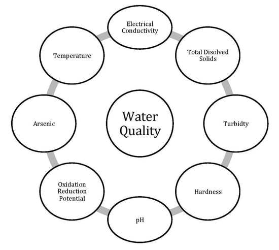
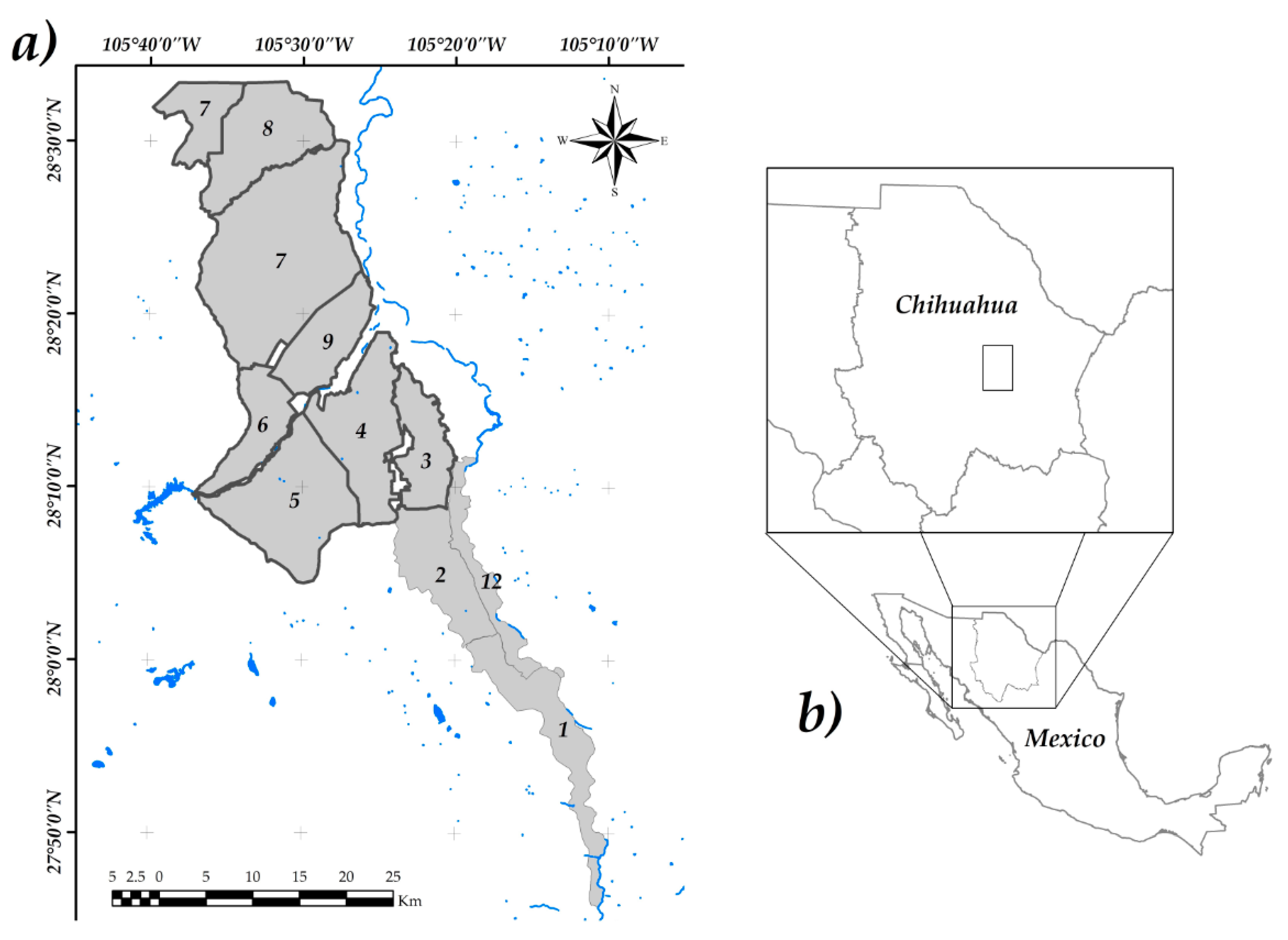
48] and many times, the studies are analyzed univariately. Therefore, the selection of PCA and CA methods was made to understand the multivariate relationship between parameters in this research, these techniques were used to compare the grouping analysis and the interpolations, to understood the spatial distribution of the parameters and even more the spatial distribution of the PCs. The objective of the present study was to analyze eight physicochemical parameters (PhP) in water samples from wells of the Irrigation District 005 (ID005) in Chihuahua, Mexico; perform a data analysis using multivariate techniques to evaluate the PhP contribution in water quality and apply interpolation methods to analyze the spatial variation of the PhP.

2. Materials and Methods

2.1. Research Area

The ID005 is located in the south-central region of the State of Chihuahua (Figure 1), among the geographical coordinates 105°40′ W–28°30′ N, 105°20′ W–28°30′ N, 105°40′ W–28°10′ N, 105°20′ W–28°10′ N. It has an average altitude of 1156 m above sea level. The predominant climate is semi-desert, with an average of annual rainfall of 350 mm [49]. The ID005 is composed by 10 irrigation modules, which are administered by local associations. The district is divided into two constituted irrigation units based on infrastructure characteristics, to facilitate water distribution [50]. Each unit is managed by a Limited Liability Corporation (Chihuahua, Mexico), that is integrated as follows: (1) The first unit called Conchos is composed by irrigation modules from 1 to 5 and module 12, which are mainly supplied by water from La Boquilla Dam; (2) The second unit, called San Pedro, is integrated by modules 6, 7, 8 and 9, which are supplied by water from the Francisco I. Madero dam, groundwater and, to a lesser extent, by water from the La Boquilla Dam [51].

2.2. Sampling

Two different sampling periods were performed in operating wells, on the studied area during 2016. The first sampling was performed in Summer (S1) and the second sampling in Fall (S2) (Figure 2), following the standard procedures of NOM-014-SSA1-1993 [52]. Two samples of 1 L were collected, one for PhP determination, and another for Arsenic (As) determination in which 2 mL of nitric acid (HNO3) were added for its preservation. The samples were transported in coolers, taken to the laboratory and stored at 4 °C until their analysis. In the first period (S1), water samples were collected of 65 wells; while in the second period (S2), of 54 wells.

2.3. Physicochemical Parameters (PhP) Analysis

For As determination, the samples were filtered with 0.2 mm ash paper Whatman No. 41 (CTR Scientific, Chihuahua, Mexico). Subsequently, before the analysis, filtered with 0.45 μm Millipore filters (CTR Scientific, Chihuahua, Mexico). The As quantification was perform in an Atomic Absorption Spectrophotometer AAnalyst 700 (Perkin Elmer, Waltham, USA) to which the FIAS 100 Hydride Generator (Perkin Elmer, Waltham, USA) was coupled, following the NMX-AA-051-SCFI-2001 [53]. The detection limit of the equipment was 3.12 μg/L. The samples were analyzed in triplicate using the standard Trace Metals-Sand 1 Number CRM048 Sigma Aldrich (CTR Scientific, Chihuahua, Mexico) with a recovery percentage of 99%.
Moreover, different physicochemical parameters (PhP) were analyzed: Temperature, Electrical Conductivity (EC), Oxide Reduction Potential (ORP), Hardness, pH, Total Dissolved Solids (TDS) and Turbidity. These are listed in Table 1 along with their respective analytical method. All parameters were analyzed in triplicate. Temperature, pH and ORP were determined in situ, the rest in the laboratory.

2.4. Multivariate Statistical Methods

Prior to the multivariate analysis, a Pearson correlation analysis was performed to understand the relationships among the PhP. To know the magnitude of the relationship between the parameters, the Pearson value is classified in 33 percentiles. The values of Pearson’s linear correlation coefficient were classified as: Poor (0.0–0.3), Moderate (0.4–0.6) and Strong (0.7–1.0) [1,54]. Such analysis was performed in the SAS© 9.1.3 software [55].
The multivariate analysis of the data of the ID005 was realized by the PCA and CA methods [25,56]. The PCA is a method for pattern recognition that attempts to explain the variance of a large set of correlated variables (PhP); transforming the data set into a smaller set of independent (uncorrelated) principal components (PC). SAS© 9.1.3 software was used to describe these patterns. The PCA is a dimensionality reduction technique that helps to simplify the data and make it easier to visualize by looking for a PC set [57]. The PCs are orthogonal variables calculated by multiplying the original correlated variables with a list of coefficients that can be described as shown in Equation (1):
z i j = a i 1 x 1 j + a i 2 x 2 j + + a i m x m j
where: z = the component’s coefficient, a = component weight, x = measured value of the variable, i = component number, j = sample number and m = number of variables.
The CA is an unsupervised pattern recognition technique that describes the structure of a data set [28]. The hierarchical grouping is the most common approach in which groups are formed sequentially, starting with the pair of most similar objects forming groups from the union of these objects. The Euclidean distance usually gives the similarity between two objects or groups of objects [58]. The resulting groups of objects should exhibit high internal homogeneity (within a group) and high external heterogeneity (among groups), where grouping is typically illustrated with a dendrogram [59]. The dendrogram provides a visual summary of the clustering processes, presenting an image of the groups and their proximity with a dramatic reduction in the dimensionality of the original data [60]. The CA was applied to classify the sampling sites by ascending cluster analysis with the Ward [61] criterion, using the determination coefficient R2 as a measure of explanation of variation and pseudo T2 served to confirm the number of groups [62]. It is possible to plot the pseudo values versus the number of clusters. If the values present a sudden change, the group value n + 1 that caused the change is a candidate for the number of groups to choose [63]. The CA was performed in the SAS© 9.1.3 software.

2.5. Spatial Variability of the Physicochemical Parameters (PhP)

The information of the PhP was used as input data to carry out an interpolation. To examine the spatial distribution of the studied variables, the interpolation method used was Inverse Distance Weight (IDW), available in ArcMap© 10.3 software (ESSRI, Redlands, CA, U.S.A.; https://www.esri.com/en-us/home). The interpolation, through IDW has been widely used to map the spatial distribution of water elements [2,64,65]. The IDW method uses the existing values that are around the area to estimate the concentration of the non-sampled sites. The values of the closest observations will have a greater influence than those that are further away, i.e., the influence decreases with distance [66]. Equation (2) shows the algorithm for IDW.
Z ( S 0 ) = i = 1 N λ   × Z ( S i )
where: Z(S0) = value to be estimated in the place S0, N = number of observations near to the place to estimate, λ = weight assigned to each observation to be used, decreases with distance, and Z(Si) = observed value of the place Si.

3. Results

3.1. Analysis of Physicochemical Parameters (PhP)

Table 2 shows the results obtained from the As and the PhP analysis of water samples, the maximum permissible levels (MPL) established according to Mexican regulations for each parameter, and the percentage of samples exceeding the limits.
In the two seasons, TDS was the parameter with the highest percentages of samples exceeding the MPL of the Mexican regulation (35% in S1, 39% in S2). Turbidity exceeded the MPL in S1 (29%) in more samples than S2 (12%). As concentrations were above the MPL of water for agricultural irrigation in 9% (Summer) and 13% (Fall) of the wells.

3.2. Multivariate Analysis

The correlation analysis reported the existence of significant positive and negative correlations (p > 0.05 and p < 0.0001) among the values of PhP from the first sampling (Table 3). As was positive moderately correlated with Turbidity and pH, and negative moderately correlated with hardness. EC was positive moderately correlated with TDS and Hardness; and negative moderately correlated with ORP. Regarding TDS was moderately correlated with Turbidity (negative) and Hardness (positive). Furthermore, pH and ORP were correlated positive strongly and negative moderately, with Temperature, respectively. The poor correlation between the other pairs of PhP indicates the presence of other variation sources.
In S2 (Table 4) it was observed that As was negative moderately correlated with Hardness while it was positive strongly correlated with pH. The EC was positive moderately correlated with Hardness and strongly correlated with TDS. Likewise, TDS was moderately negative correlated with Turbidity and ORP; and positive correlated with hardness.

3.3. Principal Components Analysis (PCA)

The assumption that the parameters are linearly related was verified, then the PCA was realized to explore the relationships among the eight PhP. The first four PCs in S1 explained 87% of the variance (Table 5). In S1, PC1 contributed with 34% of the variance, PC2 with 30%, while PC3 and PC4 contributed with 12% and 9%, respectively. The dominant PhP in PC1 were As, pH and Temperature. Considering Table 3, there is a significant correlation between As and pH (r = 0.44, p < 0.05). In PC2, the coefficients that contributed the most were EC, TDS and Hardness. The parameters correlated were: EC and TDS (r = 0.625, p < 0.0001), EC and Hardness (r = 0.493, p < 0.0001) and TDS with Hardness (r = 0.586, p < 0.0001). The PC3 was influenced by Turbidity and PC4 by As and ORP.
Regarding S2, 86% of the variance was explained by considering four PCs (Table 5). The components contributed with 35%, 24%, 16% and 9% to PC1, PC2, PC3 and PC4, respectively. The PC1 was influenced by EC, TDS and Hardness with weak coefficients. These parameters strongly and moderately correlated as follows: EC and TDS (r = 0.89, p < 0.0001), EC and Hardness (r = 0.54, p < 0.0001), Hardness and TDS (r = 0.45, p < 0.05). The PC2 was influenced by As and pH, with moderate and highly correlated coefficients (r = 0.77, p < 0.0001). The PC3 explained the Turbidity and Temperature variability, with moderate to strong coefficients and PC4 was influenced by ORP. In Table 4 it was observed that there is a highly significant correlation of EC with TDS and Hardness, which indicates that these three components explain a large amount of variation in the study area.
The grouping of the sites is shown in the displacement plane of the first two PCs (Figure 3). The PhP for S1 and S2 were organized into 4 groups. Group 1: As, pH and Temperature; Group 2: EC, TDS and Hardness; Group 3: Turbidity; and Group 4: As and ORP. In regards to S2, Group 1 was composed of: Hardness, EC, TDS; Group 2: As and pH; Group 3: Turbidity and ORP; and Group 4: Temperature. Gebreyohannes et al. [68] determined in their area of study that TDS, Hardness and EC were positively associated and these were negatively associated with pH and Turbidity.
The comparison plots of PC1 vs. PC2 in each sample indicate the displacement through components 1 and 2. These components, together explain more than 60% of the total variation. As, pH and Temperature in S1 move to the right side, indicating its dominance in PC1. While in S2, only As and pH remain dominant but in PC2. Furthermore, in S1 the variables with the greatest influence in PC2 were EC, TDS and Hardness and in S2 were also EC, TDS and but in PC1. The change in the station strongly influences the way in which the parameters are expressed in the well water, which explains the displacement of the parameters between stations.

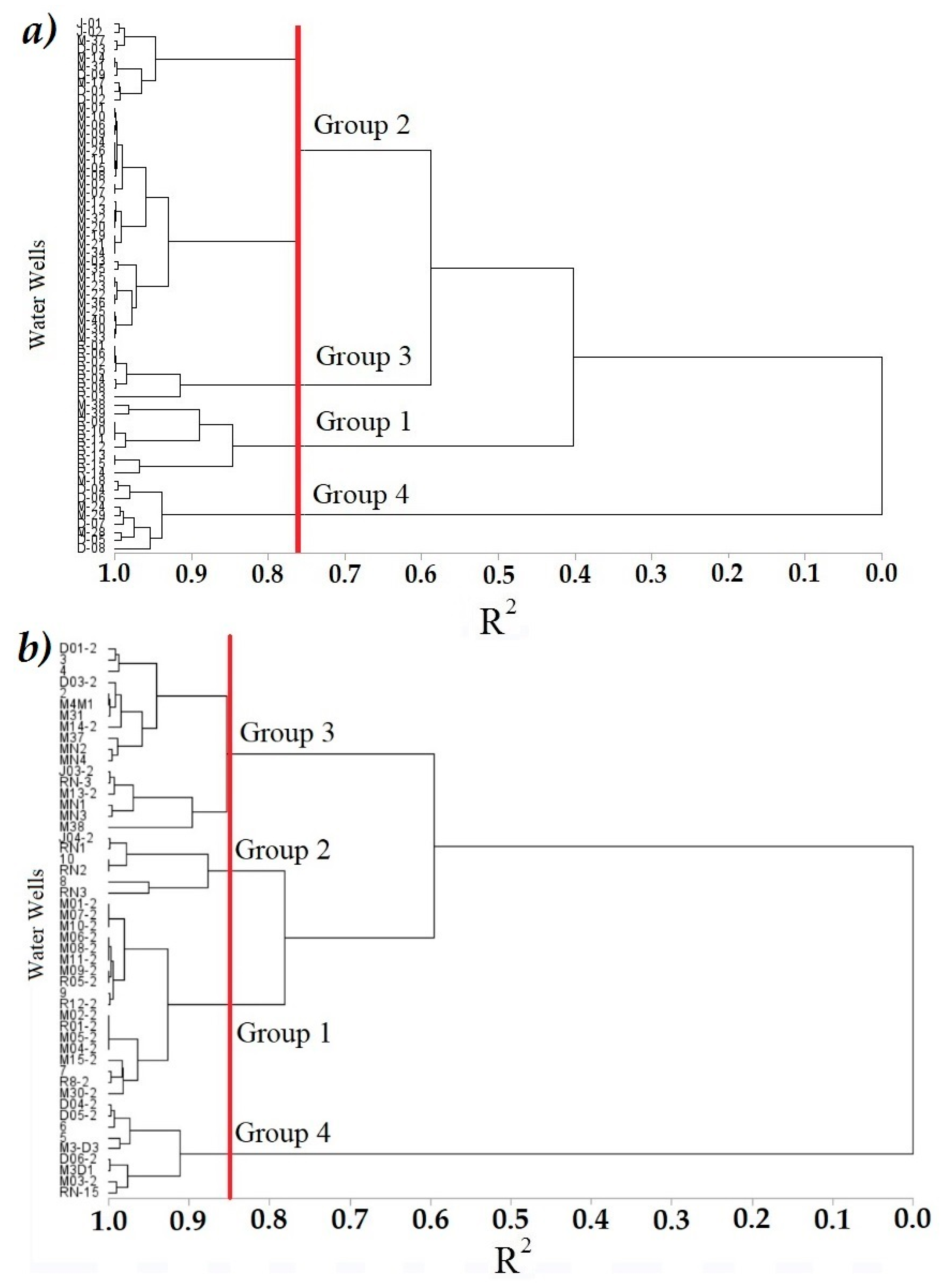
3.4. Cluster Analysis (CA)

The definition of the number of groups was made considering the value of R2 and the criterion of pseudo T2. The value of R2 indicated that, with four groups, up to 76% of the variability in S1 was explained, while in S2 with four groups 85% was explained. A line was drawn in both dendrograms to confirm the value of R2. This line is imaginary and is traced in the dendrogram to support the definition of the groups [69]. The pseudo T2 was useful to reaffirm the decision of the four groups, showing a value of 77.3 and 9.2, respectively [62]. The groups were significantly different based on the MANOVA test (F = 25.65, λ of Wilk’s = 0.002, p < 0.0001).
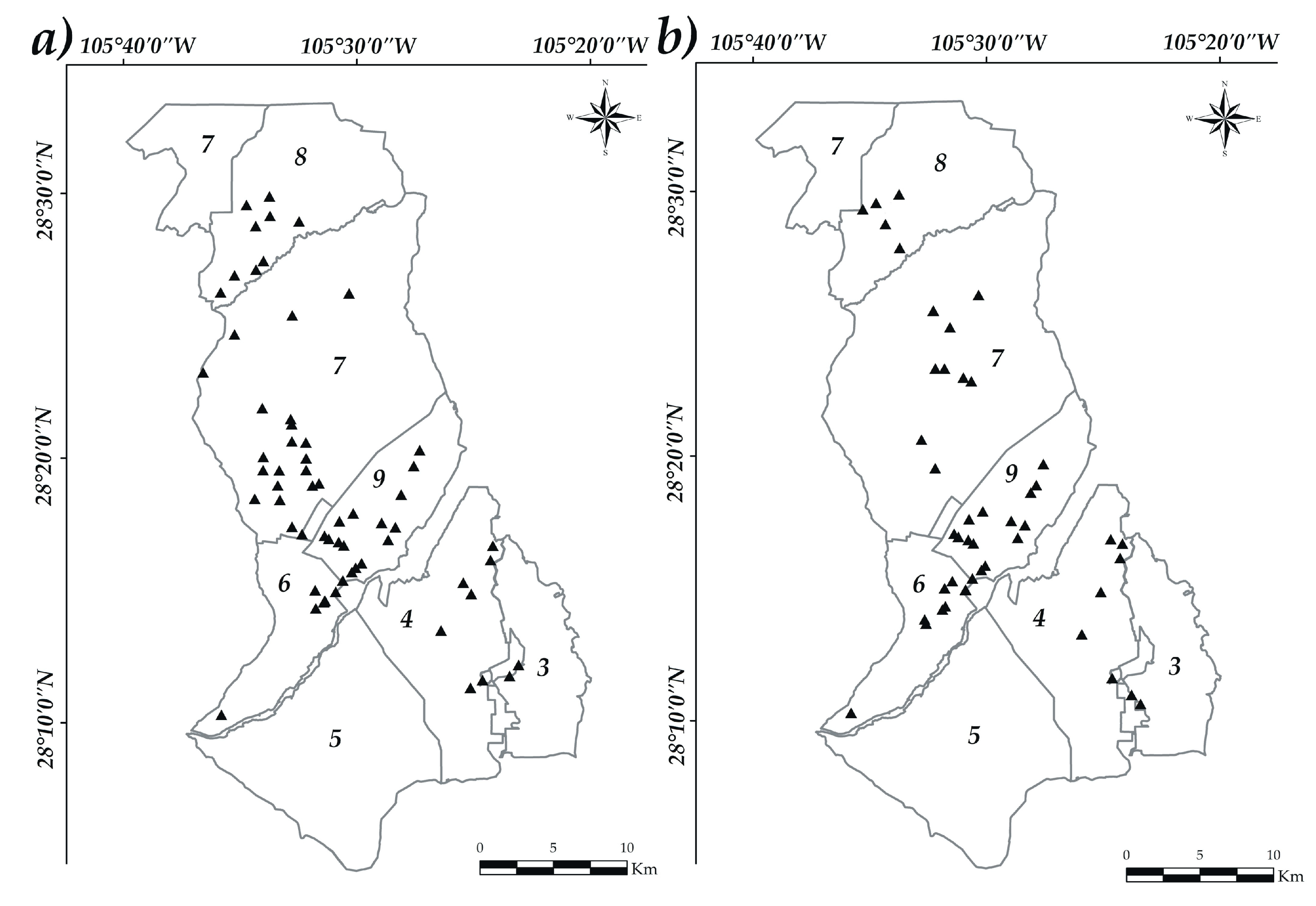
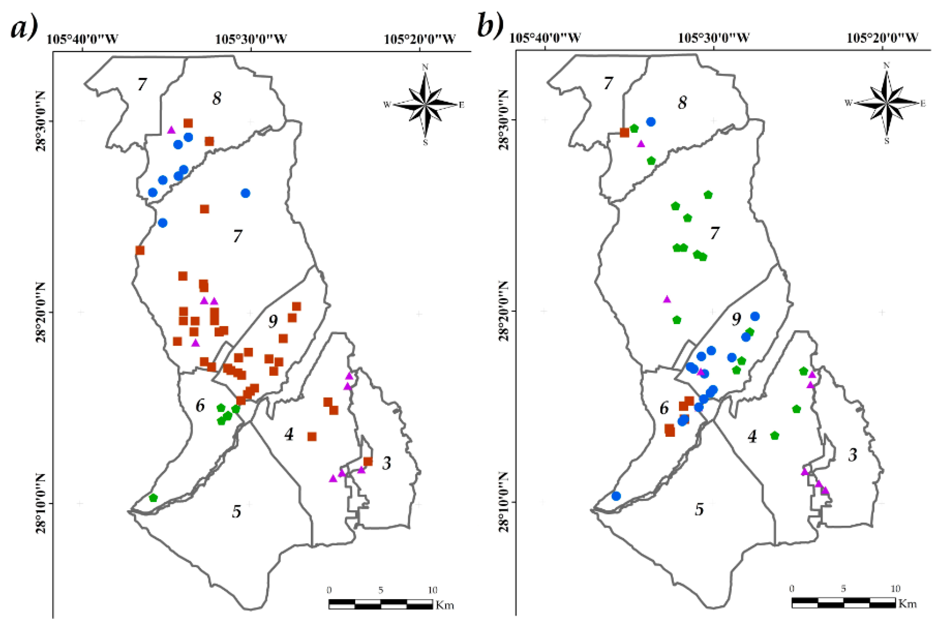
In S1, Group 1 was made up of 9 wells; Group 2 was the largest with 38 wells; Group 3, the smallest with 7 wells and Group 4 included 9 wells (Figure 4). Each group was characterized with the average of the variables per group, presented in Table 6. In S1, Group 1 consisted of high values of As (0.098 mg/L), Turbidity (687.6 NTU), pH (8.2) and EC (1117.7 μS/cm), and low values of TDS and Hardness (93.8 and 144.3 mg/L, respectively). Group 2 had moderate values with respect to almost all PhP, only with a low Turbidity value (3.9 NTU). Group 3 also presented moderate values in most of the PhP, with the exception of EC at low concentrations (15.3 μS/cm), and Turbidity at high concentrations (295.6 NTU). Lastly, Group 4 showed high values of TDS (883.9 mg/L), Hardness (497.4 mg/L), EC (1773.4 μS/cm) and Temperature (25.1 °C), while the lowest values corresponded to Turbidity (38.0 NTU). The remaining PhP had moderate values.
In the S2, Group 1 was the largest with 18 wells; Group 2 was the smallest with 6 wells; Group 3 was comprised of 17 wells; and Group 4 of 9 wells (Figure 4). Group 1 was formed with high Turbidity values (196.1 NTU). Group 2 showed the highest values of Turbidity (164.5 NTU) and the lowest values of As (0.005 mg/L) and TDS (78.9 mg/L) among all groups. Group 3 showed high values of As (0.106 mg/L), EC (1.102.5 μS/cm), TDS (563.4 mg/L), Turbidity (157.6 NTU) and pH (8.02). Finally, Group 4 had the highest values of EC (1779.1 μS/cm), TDS (885.3 mg/L), Hardness (384.7 mg/L) and the lowest Turbidity (5.2 NTU), pH (7.3) and ORP (195.2 mV) values when compared to the other groups (Table 6).
The spatial distribution of S1 and S2 was observed by linking the database derived from the CA with the vector file of wells, using ArcMap 10.3©. In S1, the distribution of Group 1 (high values of As, Turbidity and pH) was homogeneous in the northern part of the ID005, located in modules 7 and 8. Group 2, with the highest number of wells (moderate values of all PhP), included modules 4, 7, 8, 9 and 3. Group 3 (high Turbidity), was located in module 6, showing a homogeneous spatial grouping. Group 4 (high TDS, Hardness and EC) was defined in modules 4, 8, 7 and 3, being the group with the greatest geographical dispersion.
In S2, Group 1 (high Turbidity) was homogeneously distributed between module 9 and 6. Group 2 (high Turbidity) was placed in module 6, only with one observation in module 8. Group 3, with high magnitudes of As, EC, TDS, Turbidity and pH, was presented in module 7, with some observations in modules 8 and 4. Group 4, with high magnitudes of EC, TDS and Turbidity, was distributed in the boundary between module 3 and 4 in the southwest portion of the ID005 (Figure 5).

3.5. Spatial Variability of Physicochemical Parameters

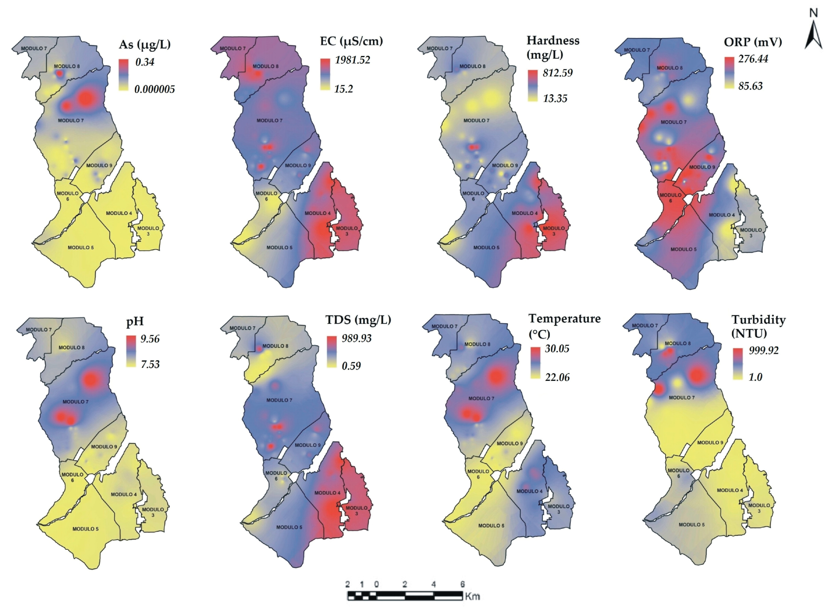
The maps of the PhP are shown in Figure 6 and Figure 7. The areas with low concentrations are colored in yellow, the blue colored areas represent moderate concentrations while the red colored areas represent high concentrations.
In S1, the PhP As, pH and Temperature showed a similar distribution where the highest and moderate concentrations are found in modules 6 and 7. The pattern of As (high concentration) may be due to a geological mineralization process [70], which seems to be present in these modules. Likewise, Hardness and TDS show a similar distribution. The highest concentrations are predominantly distributed in modules 3, 4 and 5. The EC shows a distribution pattern similar to Hardness and TDS but with some variations. The highest concentrations prevailed in modules 3, 4, 7 and 8.
In S2, As and pH showed a similar pattern with high concentrations in the northern part of module 7. The values of EC, TDS and Hardness showed a very similar spatial distribution in modules 8, 7, 4 and 3, at high concentrations. The Temperature and Turbidity PhP presented a similar pattern of high concentrations in module 6. Finally, ORP was the only variable that did not show a spatial behavior similar to the rest of the PhP.
The similarities in the spatial distribution among the PhP confirm the results of the multivariate analysis, where As-Turbidity, pH-Temperature, Hardness-TDS-EC and As-pH were grouped in S2, while TDS-EC-Turbidity were grouped in S1. In a study conducted by Li and Feng [71], similarities in the spatial distribution of the elements were found. In both, the S1 and S2 samplings, the spatial behavior for As, EC, Hardness, ORP, pH and TDS was similar. The PhP that varied were temperature and Turbidity. Temperature showed a greater variability in S1 compared to S2, which may be associated with the variation of the rest of the PhP.
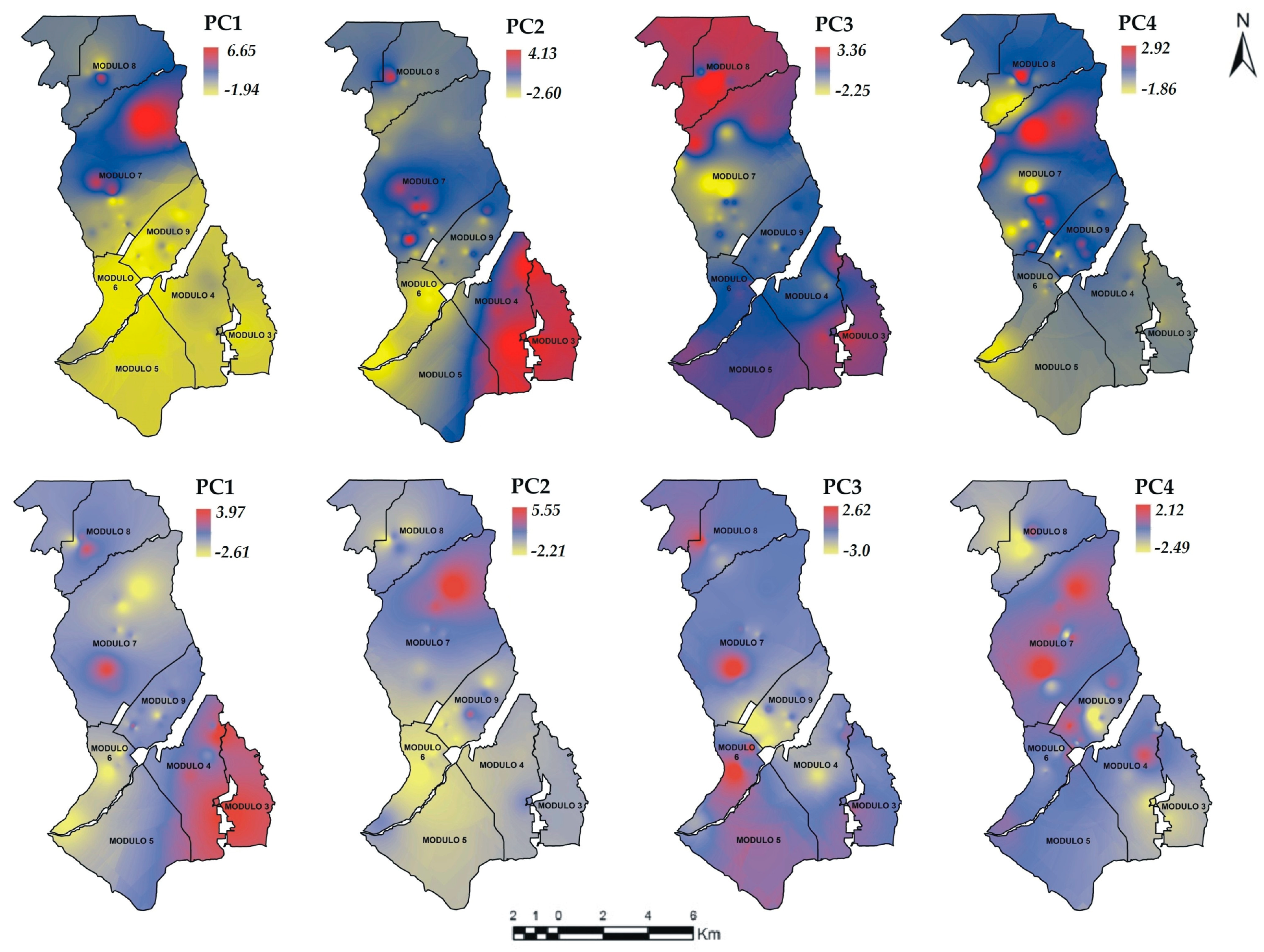
Likewise, the coefficients of each PC of the PhP were used together with the geographical coordinates of the wells to generate the interpolation of the PCs (Figure 8). These interpolations spatially indicate the multivariate relationships among the PhP.
In S1, the interpolation of the PC1 coefficients (33% of the variability explained) indicated that in the yellow areas (negative coefficients) low concentrations of As existed (0.000005 mg/L). These areas registered values of pH between 7.5–7.8 and Temperatures between 22–23 °C. Conversely, the areas in red are those with high concentrations of As (0.33 mg/L), pH (9.5) and Temperatures of 30 °C. PC2 (30%), influenced by EC, TDS and Hardness, presented negative coefficients (areas in yellow), indicating the presence of low values of EC (13–16 μS/cm), TDS (20–100 mg/L) and Hardness (100–200 mg/L). PC3 (12%), influenced by Turbidity, depicted areas with negative coefficients indicating the presence of low values for this parameter (1.0 NTU). Meanwhile, positive coefficients corresponded to areas with high concentrations (900 NTU). Although Turbidity has the highest coefficient in the matrix of eigenvectors, Temperature also shows a similar behavior in the database (not shown). In this database, the negative coefficients correspond to zones with temperatures of 30 °C and positive coefficients to areas with temperatures of 24 °C. Finally, PC4 (9%) is influenced by As and ORP. The areas with negative coefficients correspond to low concentrations of As (0.000005 mg/L) and ORP (85–113 mV). The areas in red correspond to high concentrations of As (0.27–0.34 mg/L) and ORP (250 mV).
In the S2, PC1 (35%) represents the variability of EC, TDS and Hardness. In this component, the red areas represent EC values (1863 μS/cm), TDS (932.33 mg/L) and Hardness (594 mg/L). The concentrations in yellow are for EC (1078 μS/cm), TDS (573 mg/L) and Hardness (0 mg/L), which are distributed in module 6 and the northern part of 7. PC2 (26%) explains the variability of As and pH, where the high concentrations are distributed in module 7. In this module, the coefficients with positive value indicate As concentrations of 0.575 mg/L and pH of 8.9, while in modules 6 and 5, the concentrations are the lowest (As = 0 mg/L, pH = 7.4). The distribution of PC3 (15%) explains the variation of Turbidity and Temperature. In these zones (red color), the PC explains Turbidity concentrations of 519 NTU and Temperature 23.8 °C. Turbidity values of 0.43 NTU and Temperature of 27.5 °C are reported in the yellow zones. PC4 (9%) represents the variability of ORP. The zones in red tone indicate ORP concentrations of 306 mV and in yellow values of 106 mV.

4. Discussion

The multivariate techniques and the interpolation were useful to interpret the relationship between the PhP. The PCA has been previously used to examine and interpret the behavior of groundwater quality parameters [72,73,74,75]. The relationship between the PhP provided significant information on the possible sources of these parameters. In this study, four components were needed to explain the original data set. The four components showed that the behavior of the PhP in the wells was governed by more than one process or phenomenon.
According to Yidana et al. [76], in the analysis of dimensionality reduction of variables PC1 usually represents the most important mixture of processes in the study area. The PCA results suggest that most variations in water quality were found in S1 (summer) for As, pH and Temperature followed by EC, TDS and Hardness; and in S2 (Fall) for EC, TDS and Hardness, followed by As and pH. According to Bonte et al. [77], the increase in temperatures was associated with the As increase, which was shown in S1 where the main variables that explained the total variability were shown. The above was also demonstrated in the CA and the spatial interpolation of the individual parameters and the main components where high temperature zones show a spatial distribution similar to As.
The variables that were grouped in PC1 and PC2 of each sampling season had similar coefficients, which imply the existence of some similarities in the way they influence the groundwater concentration. It was observed that As, EC, TDS, Hardness and pH were shown in components 1 and 2 in both samples. This was consistent with the results of the interpolation, showing that the distribution of these parameters had a similar dispersion in the ID005. The interpolations of the PC coefficients are similar to the maps of the main components derived from the water sampling from the wells. Previous studies have shown similar results to improve the interpretation of PC [78,79]. These variables together accounted for more than 60% of the variability of the original data set. Also, it was observed that there was an exchange of these variables in PC1 and PC2. This behavior may have been caused the result of the different sampling seasons.
These relationships agree with the natural dynamics of water PhP. The pH is the main factor that controls the concentrations of soluble metals [80]. As well as, the arid climate leads to evaporation which can interfere in the concentration of As [9] and cause seasonal variations. It was observed that As concentrations higher than the MPL (0.1 μg/L) of water for agricultural irrigation established in the Mexican regulation [67], were presented in the northern area of the territory in both S1 and S2. The EC showed a significant correlation with parameters such as Hardness, TDS [10], which can be related to water salinity [9].
In wells that contain high amounts of As, the pH is also high. This was reaffirmed by the CA method and interpolation, where Group 1 showed the highest As and pH values for S1 and S2. The first two main components (PC1 and PC2) in both seasons (S1 and S2) showed similar variations. This same behavior was observed in wells where high concentrations of EC, TDS and Hardness were obtained, which was also observed by the CA and spatial interpolation.
For this study, the wells near the city showed the highest concentrations of EC, TDS and Hardness. The EC and TDS measurements for the S1 and S2 samples showed that the salinity is classified according to the Food and Agriculture Organization of the United Nations (FAO) as moderate (EC 700–3000 μS/cm, TDS 450–2000 mg/L), especially in the southern area of ID005 [81]. EC and high TDS limit the absorption of water by crops because of the salt that stays in the roots. Due to the difficult access to water, the growth rate of plants is reduced, which limits agricultural production [61]. The EC and the TDS in groundwater samples are significantly correlated with cations and anions (Ca2+, K+, Na+, Cl+, NO3 and SO42−), which can be the result of ionic changes in the aquifer [9].
In the case of Hardness, it was within the MPL established by the Mexican regulation (500 mg/L) [52]. However, according to Gebreyohannes et al. [68], water with Hardness greater than 151 mg/L is classified as hard water. Considering these criteria, 75 and 77% of the samples (S1 and S2, respectively) were classified as hard water. This classification may indicate that there are deposits with high Mg2+ and Ca2+ contents [68]. Likewise, it is considered that hard water is not suitable for industrial and agricultural purposes [10].
The interpretation of the spatial behavior of the water quality in the studied area was possible when the scores derived from the PC were mapped. Previous studies have used geostatistical methods to map the scores resulting from PCA and used the resultant maps to predict the factors that may be impacting groundwater quality [82,83,84]. Based on the results of PCA and CA it was possible to understand the multivariate relationship of the set of parameters. In turn, with the application of the IDW interpolation technique on the scores of the PCA, it was possible to analyze the spatial variability. The combination of both methods was useful to examine patterns in common groups of parameters allowing to summarize the multiple relationship of variables on geographic regions to use in water quality analysis.
The PCA, the CA, the correlation coefficients and the interpolation were consistent with these interpretations. Although the results of the present study provided important conclusions regarding the origin of each PhP, more studies are needed to obtain a better understanding of the sources of the PhP and their concentrations.

5. Conclusions

The As is an element present in the ID005, and it is at levels that can cause a risk to agricultural production, mainly in the northern region. In addition, it is important to continue this investigation to determine the As traceability in the medium and to identify the risk of introducing this metalloid to the food chain by diet intake.
A slight issue was observed with indicators that affect the salinity of water. If such high levels persist, it can be detrimental to the optimal development of crops. Therefore, it will be necessary to look for alternatives to ameliorate this situation. Perhaps, starting with a continuous monitoring of wells in the ID005.
Multivariate statistical methods and spatial interpolation can be useful to identify locations of priority concern and potential sources of PhP, and to evaluate water quality from wells in an agricultural area. The multivariate geographic information system (GIS) approach showed the spatial relationships between the PhP (As, pH, EC, TDS and Hardness), proving to be convenient for the confirmation and refinement of PhP interpretations through the statistical results.

Author Contributions

J.A.P.-A.: sample collection, field analysis, geoinformatics and drafted the manuscript; B.A.R.-G.: carried out the physicochemical parameters in the water, evaluated the water quality in the area for irrigation and drafted the manuscript; M.d.L.B.-C.: carried out the water analysis for arsenic, data analysis and drafted the manuscript; M.C.V.-A.: conceived the study, designed of the studied area, sample collection, field analysis, processed analyzed the data, prepared the manuscript and designed the research; M.d.R.P.-P.: sample processing, statistical analysis and drafted the manuscript; A.P.-A.: contributed in the multivariate analysis and integration of geospatial information.

Funding

This research was funded by Consejo Nacional de Ciencia y Tecnología (CONACYT) of Mexico, grant CB-2014/240849, covenant I010/532/2014.

Conflicts of Interest

The authors declare no conflict of interest.

References

  1. Kengnal, P.; Megeri, M.N.; Giriyappanavar, B.S.; Patil, R.R. Multivariate Analysis for the Water Quality Assessment in Rural and Urban Vicinity of Krishna River (India). Asian J. Water Environ. Pollut. 2015, 12, 73–80. [Google Scholar]
  2. Varol, S.; Davraz, A. Evaluation of the groundwater quality with WQI (Water Quality Index) and multivariate analysis: A case study of the Tefenni Plain (Burdur/Turkey). Environ. Earth. Sci. 2015, 73, 1725–1744. [Google Scholar] [CrossRef]
  3. Qadir, A.; Malik, R.N.; Husain, S.Z. Spatio-temporal variations in water quality of Nullah Aik-tributary of the River Chenab, Pakistan. Environ. Monit. Assess. 2008, 140, 43–59. [Google Scholar] [CrossRef] [PubMed]
  4. Morris, B.L.; Lawrence, A.R.; Chilton, P.J.C.; Adams, B.; Calow, R.C.; Klinck, B.A. Groundwater and its susceptibility to degradation: A global assessment of the problem and options for management; United Nations Environment Programme: Nairobi, Kenya, 2003; Volume 3, p. 118. ISBN 92-807-2297-2. [Google Scholar]
  5. Sharma, R.K.; Agrawal, M.; Marshall, F. Heavy metal contamination of soil and vegetables in suburban areas of Varanasi, India. Ecotoxicol. Environ. Saf. 2007, 66, 258–266. [Google Scholar] [CrossRef] [PubMed]
  6. Khan, S.; Cao, Q.; Zheng, Y.M.; Huang, Y.Z.; Zhu, Y.G. Health risks of heavy metals in contaminated soils and food crops irrigated with wastewater in Beijing, China. Environ. Pollut. 2008, 152, 686–692. [Google Scholar] [CrossRef] [PubMed] [Green Version]
  7. Gupta, I.; Dhage, S.; Kumar, R. Study of variations in water quality of Mumbai coast through multivariate analysis techniques. Indian J. Mar. Sci. 2009, 38, 170–177. [Google Scholar]
  8. AlSuhaimi, A.O.; AlMohaimidi, K.M.; Momani, K.A. Preliminary assessment for physicochemical quality parameters of groundwater in Oqdus Area, Saudi Arabia. J. Saudi Soc. Agric. Sci. 2017. [Google Scholar] [CrossRef]
  9. Brahman, K.D.; Kazi, T.G.; Afridi, H.I.; Naseem, S.; Arain, S.S.; Ullah, N. Evaluation of high levels of fluoride, arsenic species and other physicochemical parameters in underground water of two sub districts of Tharparkar, Pakistan: A multivariate study. Water. Res. 2013, 47, 1005–1020. [Google Scholar] [CrossRef] [PubMed]
  10. Patil, P.N.; Sawant, D.V.; Deshmukh, R.N. Physico-chemical parameters for testing of water-A review. Int. J. Environ. Sci. 2012, 3, 1194. [Google Scholar] [CrossRef]
  11. Muangthong, S.; Shrestha, S. Assessment of surface water quality using multivariate statistical techniques: Case study of the Nampong River and Songkhram River, Thailand. Environ. Model. Assess. 2015, 187, 548. [Google Scholar] [CrossRef] [PubMed]
  12. Giri, S.; Qiu, Z. Understanding the relationship of land uses and water quality in Twenty First Century: A review. J. Environ. Manag. 2016, 173, 41–48. [Google Scholar] [CrossRef] [PubMed] [Green Version]
  13. Helena, B.; Pardo, R.; Vega, M.; Barrado, E.; Fernández, J.M.; Fernández, L. Temporal evolution of groundwater composition in an alluvial aquifer (Pisuerga river, Spain) by principal component analysis. Water Res. 2000, 34, 807–816. [Google Scholar] [CrossRef]
  14. Singh, K.P.; Malik, A.; Sinha, S. Water quality assessment and apportionment of pollution sources of Gomti river (India) using multivariate statistical techniques: A case study. Anal. Chim. Acta 2005, 538, 355–374. [Google Scholar] [CrossRef]
  15. Wang, Y.; Wang, P.; Bai, Y.; Tian, Z.; Li, J.; Shao, X.; Mustavish, L.F.; Li, B.L. Assessment of surface water quality via multivariate statistical techniques: A case study of the Songhua River Harbin region, China. J. Hydro-Environ. Res. 2013, 7, 30–40. [Google Scholar] [CrossRef]
  16. Singh, K.P.; Malik, A.; Mohan, D.; Sinha, S. Multivariate statistical techniques for the evaluation of spatial and temporal variations in water quality of Gomti River (India)—A case study. Water Res. 2004, 38, 3980–3992. [Google Scholar] [CrossRef] [PubMed]
  17. Zhao, Y.-F.; Shi, X.-Z.; Huang, B.; Dong-Sheng, Y.U.; Wang, H.-J.; Sun, W.-X.; Öboern, I.; Blombäck, K. Spatial Distribution of Heavy Metals in Agricultural Soils of an Industry-Based Peri-Urban Area in Wuxi, China. Pedosphere 2007, 17, 44–51. [Google Scholar] [CrossRef]
  18. Brogna, D.; Michez, A.; Jacobs, S.; Dufrêne, M.; Vincke, C.; Dendoncker, N. Linking forest cover to water quality: A multivariate analysis of large monitoring datasets. Water 2017, 9, 176. [Google Scholar] [CrossRef]
  19. Boyacioglu, H. Surface water quality assessment using factor analysis. Water SA 2006, 32, 389–393. [Google Scholar] [CrossRef]
  20. Bhuiyan, M.A.; Rakib, M.A.; Dampare, S.B.; Ganyaglo, S.; Suzuki, S. Surface water quality assessment in the central part of Bangladesh using multivariate analysis. KSCE. J. Civ. Eng. 2011, 15, 995–1003. [Google Scholar] [CrossRef]
  21. Batayneh, A.; Zumlot, T. Multivariate statistical approach to geochemical methods in water quality factor identification; application to the shallow aquifer system of the Yarmouk basin of North Jordan. Res. J. Environ. Earth Sci. 2012, 4, 756–768. [Google Scholar]
  22. Oketola, A.A.; Adekolurejo, S.M.; Osibanjo, O. Water quality assessment of River Ogun using multivariate statistical techniques. J. Environ. Prot. 2013, 4, 466. [Google Scholar] [CrossRef]
  23. Miranda, J.; Andrade, E.; López-Suárez, A.; Ledesma, R.; Cahill, T.A.; Wakabayashi, P.H. A receptor model for atmospheric aerosols from a southwestern site in Mexico City. Atmos. Environ. 1996, 30, 3471–3479. [Google Scholar] [CrossRef]
  24. Jackson, B.B. Multivariate Data Analysis: An Introduction; Prentice Hall: Irwin, Homewood, IL, USA, 1983; pp. 154–196. ISBN 978-0256028485. [Google Scholar]
  25. Wunderlin, D.A.; Diaz, M.P.; Ame, M.V.; Pesce, S.F.; Hued, A.C.; Bistoni, M.A. Pattern recognition techniques for the evolution of spatial and temporal variations in water quality. A case study: Suquia river basin (Cordoba-Argentina). Water Res. 2001, 35, 2881–2894. [Google Scholar] [CrossRef]
  26. Loska, K.; Wiechuła, D. Application of principal component analysis for the estimation of source of heavy metal contamination in surface sediments from the Rybnik Reservoir. Chemosphere 2003, 51, 723–733. [Google Scholar] [CrossRef]
  27. Vega, M.; Pardo, R.; Barrado, E.; Deban, L. Assessment of seasonal and polluting effects on the quality of river water by exploratory data analysis. Water Res. 1998, 32, 3581–3592. [Google Scholar] [CrossRef]
  28. Al-Bassam, A.M. Evaluation of ground water quality in Al-Qassim area, Saudi Arabia, using cluster and factor analyses. Kuwait J. Sci. Eng. 2006, 33, 101–121. [Google Scholar]
  29. Kazi, T.G.; Arain, M.B.; Jamali, M.K.; Jalbani, N.; Afridi, H.I.; Sarfraz, R.A.; Baig, J.A.; Shah, A.Q. Assessment of water quality of polluted lake using multivariate statistical techniques: A case study. Ecotoxicol. Environ. Saf. 2009, 72, 301–309. [Google Scholar] [CrossRef] [PubMed]
  30. Chiu, W.C. Modelación y Simulación Para el Drenaje de Tierras, en la Planicie Aluvial del Estado de Tabasco, México. Ph.D. Thesis, Autonomous University of Nuevo León, Marin, Nuevo León, Mexico, 2000. [Google Scholar]
  31. Medellín-Vázquez, J.J. Análisis de la Vegetación en un Gradiente Altitudinal Mediante Técnicas Multivariadas, en el Campo Santa María, Lampazos de Naranjo, Nuevo León y Candela Coahuila. Master Thesis, Autonomous University of Nuevo León, Linares, Nuevo León, México, 2003. [Google Scholar]
  32. Villatoro, M.; Henríquez, C.; Sancho, F. Comparación de los interpoladores IDW y Kriging en la variación espacial de pH, Ca, CICE y P del suelo. Agron. Costarric. 2008, 32, 95–105. [Google Scholar]
  33. Bhunia, G.S.; Shit, P.K.; Maiti, R. Comparison of GIS-based interpolation methods for spatial distribution of soil organic carbon (SOC). J. Saudi Soc. Agric. Sci. 2016. [Google Scholar] [CrossRef]
  34. Xie, Y.; Chen, T.B.; Lei, M.; Yang, J.; Guo, Q.J.; Song, B.; Zhou, X.Y. Spatial distribution of soil heavy metal pollution estimated by different interpolation methods: Accuracy and uncertainty analysis. Chemosphere 2011, 82, 468–476. [Google Scholar] [CrossRef] [PubMed]
  35. Yan, W.; Mahmood, Q.; Peng, D.; Fu, W.; Chen, T.; Wang, Y.; Li, S.; Chen, J.; Liu, D. The spatial distribution pattern of heavy metals and risk assessment of moso bamboo forest soil around lead–zinc mine in Southeastern China. Soil Till. Res. 2015, 153, 120–130. [Google Scholar] [CrossRef]
  36. Navarrete Álvarez, M. Modelos Geoestadísticos del Precio de la Vivienda: Aproximación al Conocimiento Intraurbano de la Ciudad de Madrid. Ph.D. Thesis, Autonomous University of Madrid, Madrid, Spain, 2012. [Google Scholar]
  37. Wang, S.; Huang, G.H.; Lin, Q.G.; Li, Z.; Zhang, H.; Fan, Y.R. Comparison of interpolation methods for estimating spatial distribution of precipitation in Ontario, Canada. Int. J. Climatol. 2014, 34, 3745–3751. [Google Scholar] [CrossRef]
  38. Núñez López, D.; Treviño Garza, E.J.; Reyes Gómez, V.M.; Muñoz Robles, C.A.; Aguirre Calderón, O.A.; Jiménez Pérez, J. Uso de modelos de regresión para interpolar espacialmente la precipitación media mensual en la cuenca del río Conchos. Rev. Mex. Cienc. Agríc. 2014, 5, 201–213. [Google Scholar]
  39. Skeppström, K.; Olofsson, B. A prediction method for radon in groundwater using GIS and multivariate statistics. Sci. Total Environ. 2006, 367, 666–680. [Google Scholar] [CrossRef] [PubMed]
  40. Maroju, S. Evaluation of five GIS-based interpolation techniques for estimating the radon concentration for unmeasured zip codes in the state of Ohio. Master Thesis, University of Toledo, Toledo, OH, USA, 2007. [Google Scholar]
  41. Johnston, K.; Ver Hoef, J.M.; Krivoruchko, K.; Lucas, N. Using ArcGIS Geostatistical Analyst; Redlands ESRI: Redlands, CA, USA, 2001. [Google Scholar]
  42. Behera, S.K.; Shukla, A.K. Spatial distribution of surface soil acidity, electrical conductivity, soil organic carbon content and exchangeable potassium, calcium and magnesium in some cropped acid soils of India. Land Degrad. Dev. 2015, 26, 71–79. [Google Scholar] [CrossRef]
  43. Markus, J.; McBratney, A.B. A review of the contamination of soil with lead II. Spatial distribution and risk assessment of soil lead. Environ. Int. 2001, 27, 399–411. [Google Scholar] [CrossRef]
  44. Rawlins, B.G.; Lark, R.M.; Webster, R.; O’Donnell, K.E. The use of soil survey data to determine the magnitude and extent of historic metal deposition related to atmospheric smelter emissions across Humberside, UK. Environ. Pollut. 2006, 143, 416–426. [Google Scholar] [CrossRef] [PubMed]
  45. Maas, S.; Scheifler, R.; Benslama, M.; Crini, N.; Lucot, E.; Brahmia, Z.; Benyacoub, S.; Giraudoux, P. Spatial distribution of heavy metal concentrations in urban, suburban and agricultural soils in a Mediterranean city of Algeria. Environ. Pollut. 2010, 158, 2294–2301. [Google Scholar] [CrossRef] [PubMed]
  46. Walter, A.M.; Christensen, S.; Simmelsgaard, S.E. Spatial correlation between weed species densities and soil properties. Weed Res. 2002, 42, 26–38. [Google Scholar] [CrossRef]
  47. Chaoyang, W.E.I.; Cheng, W.A.N.G.; Linsheng, Y.A.N.G. Characterizing spatial distribution and sources of heavy metals in the soils from mining-smelting activities in Shuikoushan, Hunan Province, China. J. Environ. Sci. 2009, 21, 1230–1236. [Google Scholar]
  48. Fu, S.; Wei, C.Y. Multivariate and spatial analysis of heavy metal sources and variations in a large old antimony mine, China. J. Soil Sediments 2013, 13, 106–116. [Google Scholar] [CrossRef]
  49. Ortega-Gaucin, D.; Mejía Sáenz, E.; Palacios Vélez, E.; Rendón Pimentel, L.; Exebio García, A. Modelo de optimización de recursos para un distrito de riego. Terra Latinoamericana 2009, 27, 219–226. [Google Scholar]
  50. Aguirre-Grijalva, E. Estudio de Factibilidad Técnica y Económica de 3 Métodos de Tecnificación del Riego en el Modulo 07 del Distrito 005. Master Thesis, Instituto Tecnológico de la Construcción, Chihuahua, Mexico, 2003. [Google Scholar]
  51. Ortega-Gaucin, D. Reglas de operación para el sistema de presas del Distrito de Riego 005 Delicias, Chihuahua, México. Ing. Agric. Biosist. 2012, 4, 31–39. [Google Scholar] [CrossRef]
  52. SSA (Secretaría de Salud) 1993. NOM-014-SSA1. Procedimientos Sanitarios para el Muestreo de Agua para Uso y Consumo Humano en Sistemas de Abastecimiento de Agua Públicos y Privados. Available online: http://www.salud.gob.mx/unidades/cdi/nom/014ssa13.html (accessed on 15 May 2017).
  53. SCFI (Secretaría de Comercio y Fomento Industrial) 2001. NMX-AA-051-SCFI. Análisis de Agua Medición de Metales por Absorción Atómica en Aguas Naturales, Potables, Residuales y Residuales Tratadas—Método de Prueba. Available online: http://www.economia-nmx.gob.mx/normas/nmx/2010/nmx-aa-051-scfi-2016.pdf (accessed on 15 May 2017).
  54. Jothivenkatachalam, K.; Nithya, A.; Chandra, M.S. Correlation analysis of drinking water quality in and around Perur block of Coimbatore District, Tamil Nadu, India. Rasayan J. Chem. 2010, 3, 649–654. [Google Scholar]
  55. SAS (Statistical Analysis Software) Institute. SAS Software; Version 9.1.3; SAS Inc.: Cary, NC, USA, 2006. [Google Scholar]
  56. Simeonov, V.; Stratis, J.A.; Samara, C.; Zachariadis, G.; Voutsa, D.; Anthemidis, A. Assessment of the surface water quality in Northern Greece. Water Res. 2003, 37, 4119–4124. [Google Scholar] [CrossRef]
  57. Jolliffe, I.T. Principal Component Analysis, 2nd ed.; John Wiley & Sons Inc.: Charlottesville, VA, USA, 2002; pp. 150–166. ISBN 978-0-387-22440-4. [Google Scholar]
  58. Otto, M. Multivariate methods. In Analytical Chemistry; Kellner, R., Mermet, J.M., Otto, M., Widmer, H.M., Eds.; Wiley-VCH: Weinheim, Germany, 1998; p. 916. ISBN 3-527-28881-3. [Google Scholar]
  59. Shrestha, S.; Kazama, F. Assessment of surface water quality using multivariate statistical techniques: A case study of the Fuji River Basin, Japan. Environ. Model. Softw. 2007, 22, 464–475. [Google Scholar] [CrossRef]
  60. McKenna, J.E., Jr. An enhanced cluster analysis program with bootstrap significance testing for ecological community analysis. Environ. Model. Softw. 2003, 18, 205–220. [Google Scholar] [CrossRef]
  61. Ward, J.H., Jr. Hierarchical grouping to optimize an objective function. J. Am. Stat. Assoc. 1963, 58, 236–244. [Google Scholar] [CrossRef]
  62. Eder, B.K.; Davis, J.M.; Bloomfield, P. An automated classification scheme designed to better elucidate the dependence of ozone on meteorology. J. Appl. Meteorol. 1994, 33, 1182–1199. [Google Scholar] [CrossRef]
  63. Neil, H.T. Applied Multivariate Analysis, 1st ed.; Springer: Board, NY, USA, 2002; p. 532. ISBN 0-387-95347-7. [Google Scholar]
  64. Arslan, H.; Turan, N.A. Estimation of spatial distribution of heavy metals in groundwater using interpolation methods and multivariate statistical techniques; its suitability for drinking and irrigation purposes in the Middle Black Sea Region of Turkey. Environ. Monit. Assess. 2015, 187, 516. [Google Scholar] [CrossRef] [PubMed]
  65. Ishaku, J.M.; Ankidawa, B.A.; Pwalas, A.J.D. Evaluation of Groundwater Quality Using Multivariate Statistical Techniques, in Dashen Area, North Eastern Nigeria. Br. J. Appl. Sci. Technol. 2016, 14. [Google Scholar] [CrossRef]
  66. Moreno, J.A. Sistemas y Análisis de la Información Geográfica. Manual de Autoaprendizaje con ArcGIS, 2nd ed.; Ra-Ma: Madrid, Spain, 2008; p. 908. ISBN 978-84-7897-838-0. (In Spanish) [Google Scholar]
  67. CONAGUA (Comisión Nacional del Agua) 2017. Ley Federal de Derechos Disposiciones Aplicables en Materia de Aguas Nacionales. Available online: https://www.gob.mx/cms/uploads/attachment/file/105138/Ley_Federal_de_Derechos.pdf (accessed on 21 June 2017).
  68. Gebreyohannes, F.; Gebrekidan, A.; Hedera, A.; Estifanos, S. Investigations of physico-chemical parameters and its pollution implications of Elala River, Mekelle, Tigray, Ethiopia. Momona Ethiop. J. Sci. 2015, 7, 240–257. [Google Scholar] [CrossRef]
  69. Güler, C.; Thyne, G.D.; McCray, J.E.; Turner, K.A. Evaluation of graphical and multivariate statistical methods for classification of water chemistry data. Hydrogeol. J. 2002, 10, 455–474. [Google Scholar] [CrossRef]
  70. Bu, J.; Sun, Z.; Zhou, A.; Xu, Y.; Ma, R.; Wei, W.; Liu, M. Heavy Metals in Surface Soils in the Upper Reaches of the Heihe River, Northeastern Tibetan Plateau, China. Int. J. Environ. Res. Public Health 2016, 13, 247. [Google Scholar] [CrossRef] [PubMed]
  71. Li, X.; Feng, L. Multivariate and geostatistical analyzes of metals in urban soil of Weinan industrial areas, Northwest of China. Atmos. Environ. 2012, 47, 58–65. [Google Scholar] [CrossRef]
  72. Sánchez-Martos, F.; Jiménez-Espinosa, R.; Pulido-Bosch, A. Mapping groundwater quality variables using PCA and geostatistics: A case study of Bajo Andarax, Southeastern Spain. Hydrol. Sci. J. 2001, 46, 227–242. [Google Scholar] [CrossRef]
  73. Liu, C.-W.; Lin, K.-H.; Kuo, Y.-M. Application of factor analysis in the assessment of groundwater quality in a blackfoot disease area in Taiwan. Sci. Total. Environ. 2003, 313, 77–89. [Google Scholar] [CrossRef]
  74. Chapagain, S.K.; Pandey, V.P.; Shrestha, S.; Nakamura, T.; Kazama, F. Assessment of deep groundwater quality in Kathmandu Valley using multivariate statistical techniques. Water Air Soil Pollut. 2010, 210, 277–288. [Google Scholar] [CrossRef]
  75. Belkhiri, L.; Boudoukha, A.; Mouni, L. A multivariate statistical analysis of groundwater chemistry data. Int. J. Environ. Res. 2011, 5, 537–544. [Google Scholar]
  76. Yidana, S.M.; Banoeng-Yakubo, B.; Akabzaa, T.M. Analysis of groundwater quality using multivariate and spatial analyses in the Keta basin, Ghana. J. Afr. Earth Sci. 2010, 58, 220–234. [Google Scholar] [CrossRef]
  77. Bonte, M.; van Breukelen, B.M.; Stuyfzand, P.J. Temperature-induced impacts on groundwater quality and arsenic mobility in anoxic aquifer sediments used for both drinking water and shallow geothermal energy production. Water Res. 2013, 47, 5088–5100. [Google Scholar] [CrossRef] [PubMed]
  78. Lu, A.; Wang, J.; Qin, X.; Wang, K.; Han, P.; Zhang, S. Multivariate and geostatistical analyses of the spatial distribution and origin of heavy metals in the agricultural soils in Shunyi, Beijing, China. Sci. Total Environ. 2012, 425, 66–74. [Google Scholar] [CrossRef] [PubMed] [Green Version]
  79. Mueller, U.A.; Grunsky, E.C. Multivariate spatial analysis of lake sediment geochemical data; Melville Peninsula, Nunavut, Canada. Appl. Geochem. 2016, 75, 247–262. [Google Scholar] [CrossRef]
  80. Acosta, J.A.; Faz, A.; Martínez-Martínez, S.; Zornoza, R.; Carmona, D.M.; Kabas, S. Multivariate statistical and GIS-based approach to evaluate heavy metals behavior in mine sites for future reclamation. J. Geochem. Explor. 2011, 109, 8–17. [Google Scholar] [CrossRef]
  81. Ayers, R.S.; Westcot, D.W. Water Quality for Agriculture; Food and Agriculture Organization of the United Nations: Rome, Italy, 1994. [Google Scholar]
  82. Kolsi, S.H.; Bouri, S.; Hachicha, W.; Dhia, H.B. Implementation and evaluation of multivariate analysis for groundwater hydrochemistry assessment in arid environments: A case study of Hajeb Elyoun–Jelma, Central Tunisia. Environ. Earth Sci. 2013, 70, 2215–2224. [Google Scholar] [CrossRef]
  83. De Freitas Alves, S.M.; de Queiroz, D.M.; de Alcântara, G.R.; dos Reis, E.F. Spatial Variability of Physical and Chemical Attributes of Soil Using Techniques of Principal Component Analysis. Biosci. J. 2014, 30, 22–30. [Google Scholar]
  84. Ha, H.; Olson, J.R.; Bian, L.; Rogerson, P.A. Analysis of heavy metal sources in soil using kriging interpolation on principal components. Environ. Sci. Technol. 2014, 48, 4999–5007. [Google Scholar] [CrossRef] [PubMed]
Figure 1. Geographical location of the study area: (a) Irrigation District 005 location (), boundary of the studied area (), water bodies (), bold numbers denote the module number, (b) Irrigation District 005 location in Chihuahua, Mexico.
Water 10 01037 g001
Figure 2. Sampling maps: (a) Summer (Sampling 1—left) and (b) Fall (Sampling 2—right). Studied modules (), sampling points ( Water 10 01037 i001), bold numbers denote the module number.
Water 10 01037 g002
Figure 3. Plot S1 comparison PC1 vs. PC2 (a), Plot S2 comparison PC1 and PC2 (b).
Water 10 01037 g003
Figure 4. Dendogram. Grouping of sampling sites according to the PhP of the ID005 for S1 (a) and S2 (b).
Water 10 01037 g004
Figure 5. Spatial distribution of the groups in the IDDR005. S1 (a), S2 (b). Group 1 (), Group 2 (), Group 3 ( Water 10 01037 i002), Group 4 (), bold numbers denote the module number.
Water 10 01037 g005
Figure 6. Spatial distribution of the PhP in the ID005 for S1. As = Arsenic, EC = Electrical Conductivity, pH = pH, ORP = Oxide Reduction Potential, studied modules (—).
Water 10 01037 g006
Figure 7. Spatial distribution of the PhP in the ID005 for S2, As = Arsenic, EC = Electrical Conductivity, pH = pH, ORP = Oxide Reduction Potential, studied modules (—).
Water 10 01037 g007
Figure 8. Spatial distribution of the PC scores of S1 (top) and S2 (bottom). PC = Principal component, studied modules (—).
Water 10 01037 g008
Table 1. Physicochemical parameters in water, units, and analytical method.
ParameterUnitAnalytical Method
Asmg/LAAS Perkin Elmer Aanalist 700, coupled HG FIAS 100
Temp°CPotentiometer Hanna portable (in situ)
ECµS/cmElectrical conductivity meter CYBERSCAN
ORPmVPotentiometer Hanna portable (in situ)
Hardnessmg/LTitration net NET (indicator)
pHdimensionlessPotentiometer Hanna portable (in situ)
TDSmg/LElectrical conductivity meter CYBERSCAN
TurbNTUElectrical conductivity meter CYBERSCAN
As = Arsenic, EC = Electrical Conductivity, Turb = Turbidity, pH = pH, ORP = Oxide Reduction Potential, Temp = Temperature, Potentiometer Hanna portable (CTR Scientific, Chihuahua, Mexico), Electrical conductivity meter CYBERSCAN (FESTA, Chihuahua, Mexico), Titration net NET (indicator) (FESTA, Chihuahua, Mexico).
Table 2. Range of PhP concentrations, maximum permissible levels and percentage of samples that exceed it.
ParameterConcentration Range S1Concentration Range S2MPLNormativeAbove MPL S1 (%)Above MPL S2 (%)
As (mg/L)ND–0.338ND–0.5760.100[67]913
Temp (°C)22.1–30.122.8–27.5-Without regulation--
EC (μS/cm)13.8–1981.6553.6–2600-Without regulation--
ORP (mV)85.6–267.798.1–306.3-Without regulation--
Hardness (mg/L)13.3–8140–611500[52]95
pH7.5–9.67.3–9.06.0–9.0[67]1.50
TDS (mg/L)0–9900–932.3500[67]3539
Turb (NTU)0–10000.2–51910[67]2912
As = Arsenic, EC = Electrical Conductivity, Turb = Turbidity, pH = pH, ORP = Oxide Reduction Potential, Temp = Temperature. MPL = Maximum permissible level.
Table 3. Pearson correlation among the PhP in the wells of the ID005, sampling 1 (S1).
AsECTDSTurbHardnesspHORPTemp
As1.00
EC0.071.00
TDS−0.170.625 **1.00
Turb0.42−0.01−0.452 **1.00
Hardness−0.477 **0.493 **0.586 **−0.231.00
pH0.441 *0.08−0.040.17−0.348 *1.00
ORP−0.092 *−0.44−0.17−0.18−0.09−0.398 *1.00
Temp0.389 *0.327 *0.230.13−0.170.827 **−0.462 *1.00
As = Arsenic, EC = Electrical Conductivity, Turb = Turbidity, pH = pH, ORP = Oxide Reduction Potential, Temp = Temperature, * = Significant p > 0.05, ** = Highly significant p > 0.0001.
Table 4. Pearson correlation among the PhP in the wells of the ID005, sampling 2 (S2).
AsECTDSTurbHardnesspHORPTemp
As1
EC−0.021
TDS0.080.89 **1
Turb−0.14−0.2−0.55 **1
Hardness−0.46 *0.54 **0.45 *−0.151
pH0.77 **−0.14−0.03−0.07−0.60 **1
ORP0.03−0.33 *−0.41 *0.32 *−0.13−0.041
Temp−0.25−0.19−0.06−0.210.04−0.29 *−0.041
As = Arsenic, EC = Electrical Conductivity, Turb = Turbidity, pH = pH, ORP = Oxide Reduction Potential, Temp = Temperature, * = Significant p > 0.05, ** = Highly significant p > 0.0001.
Table 5. Eigenvectors and eigenvalues of the PhP.
PhPS1S2
PC1PC2PC3PC4PC1PC2PC3PC4
As0.441−0.110.1080.661−0.220.560.000.24
EC0.0660.5330.3120.2610.490.210.310.07
TDS−0.130.544−0.190.3180.500.320.030.17
Turb0.305−0.190.7270.011−0.28−0.270.53−0.31
Hardness−0.330.4240.263−0.030.47−0.230.200.16
pH0.5180.1−0.34−0.16−0.280.55−0.02−0.03
ORP−0.29−0.33−0.260.604−0.29−0.220.260.87
Temp0.480.271−0.27−0.040.06−0.26−0.720.17
Eigenvalue2.7082.4731.0310.7572.82.151.240.75
Variability0.3380.3090.1280.0940.350.260.150.09
Cumulative0.3380.6470.7760.8710.350.620.770.86
As = Arsenic, EC = Electrical Conductivity, Turb = Turbidity, pH = pH, ORP = Oxide Reduction Potential, Temp = Temperature, Bold letters indicate the dominant coefficients.
Table 6. Average value of the PhP by groups.
GS1S2
AsECTDSTurbHardnesspHORPTempAsECTDSTurbHardnesspHORPTemp
10.0981117.6593.84687.63144.348.21150.2925.250.017686.111344.5528.182196.0747.701231.45624.796
20.035832.62415.063.89208.067.98208.5724.420.005768.71778.938382.933164.5337.665270.15623.856
30.01415.25185.71295.56207.037.53230.0822.590.1061102.486563.3715.753157.6478.024210.41824.170
40.0081773.36883.9138.01497.417.77138.6625.070.0051779.137885.2785.228384.6787.525195.21924.203
G = Group, As = Arsenic, EC = Electrical Conductivity, Turb = Turbidity, pH = pH, ORP = Oxide Reduction Potential, Temp = Temperature.

