Dry Pipes: Associations between Utility Performance and Intermittent Piped Water Supply in Low and Middle Income Countries

Abstract

Intermittent piped water supply impacts at least one billion people around the globe. Given the environmental and public health implications of poor water supply, there is a strong practical need to understand how and why intermittent supply occurs, and what strategies may be used to move utilities towards the provision of continuous water supply. Leveraging data from the International Benchmarking Network for Water and Sanitation Utilities, we discover 42 variables that have statistically significant associations with intermittent water supply at the utility scale across 2115 utilities. We categorized these under the following themes: Physical infrastructure system scale, coverage, consumer type, public water points, financial, and non-revenue water and metering. This research identifies globally relevant factors with high potential for cross-context, scaled impact. In addition, using insights from the analysis, we provide empirically grounded recommendations and data needs for improved global indicators of utility performance related to intermittent supply.

1. Introduction

An estimated one billion people around the world receive piped water that is available for fewer than 24 h every day, in what is often called intermittent water supply (IWS) [1,2]. IWS is a widespread mode of operation for piped systems in both urban and rural contexts across all populated regions of the world. Functionally, utilities with this mode of operation may supply water for all but a few hours per day, or may only supply water for a few hours per week [2]. While there have been initiatives to transition utilities from intermittent to continuous supply, many of these have remained in pilot phases [3]. In addition, and more alarmingly, there is evidence that average hours of supply provided by piped systems may be declining in many places, even as access to piped water is increasing globally [4].

IWS has serious practical implications for consumers, as it can lead to poorer water quality, lower water quantities, adverse health impacts, and increased costs [5,6,7,8,9]. IWS can also have negative consequences for utility operation, such as cycling pressures in pipe networks that may increase system maintenance requirements [10,11,12,13]. In addition, lower reliance on municipal piped water by consumers can lead to shrinking demands, lower cost-recovery, and a further decline in service [14,15]. Indeed, some have hypothesized that utilities can fall into a ‘low-level equilibrium trap’, with a negative feedback loop created between poor utility performance and low willingness to pay for water, leading to low cost-recovery and continually declining performance [16,17,18]. From this perspective, IWS is one component of a complex negative feedback loop that has the potential to devolve toward ever lower hours of supply, water quality, and overall service levels. Galaitsi et al. identified the conditions of IWS and pathways between them that reinforced this spiral, including large-scale trends, local governance, capacity constraints, consumer responses, and health [19]. Similarly, Totsuka et al. [20] put forth several theories for the causes of intermittency, including scarcity from poor management, economic scarcity, and absolute water scarcity. Recent analyses of failure of rural water supplies have highlighted the interrelations between social, financial, institutional, and management systems, and the importance of considering multiple types of water system failures [21,22,23]. However, while past work provides insights into the reasons for intermittency and, more broadly, water supply failure, there have been few empirical studies examining relationships between the complexities of the factors playing into utility performance in general and IWS in particular.

As such, the objective of this study is to identify associations between utility benchmarking data and hours of supply. To do so, we use World Bank data from the International Benchmarking Network, which is the largest existing database of standardized information on utility demographics and performance. Any statistically significant relationships discovered here can then be used as a screening tool for future and more localized research that can problematize the statistically observed relationships and seek the mechanisms behind them. This approach enables researchers and utilities to identify and target globally relevant strategies that have empirically demonstrated potential to scale. By exploring a wide range of factors that may affect hours of supply, it may be possible to systematically identify strategies that can be used to increase hours of supply and thus deliver better water supply to the global public.

2. Materials and Methods

The International Benchmarking Network (IBNET) [24] collects standardized, comparative cost and performance information from water supply and sanitation utilities around the globe. For example, the data categories include country information, utility and service area information, water services, investment information, institutional development data, sewerage services, financial information, tariff information, affordability information, and poverty indicators. The dataset includes both raw data (as entered by utilities or data recorders) and indicators, which are calculated or derived from the raw data. For example, the number of people served by the water supply and the number of people residing in the supply area are described as raw data, but the percent of people served by the utility is a corresponding indicator calculated from these two raw data points. A detailed description of each variable may be obtained from [25].

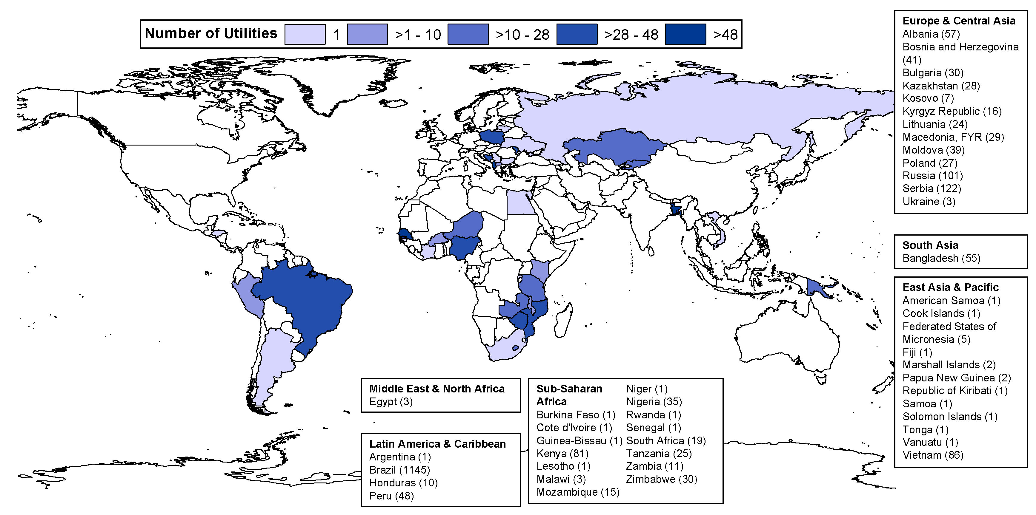
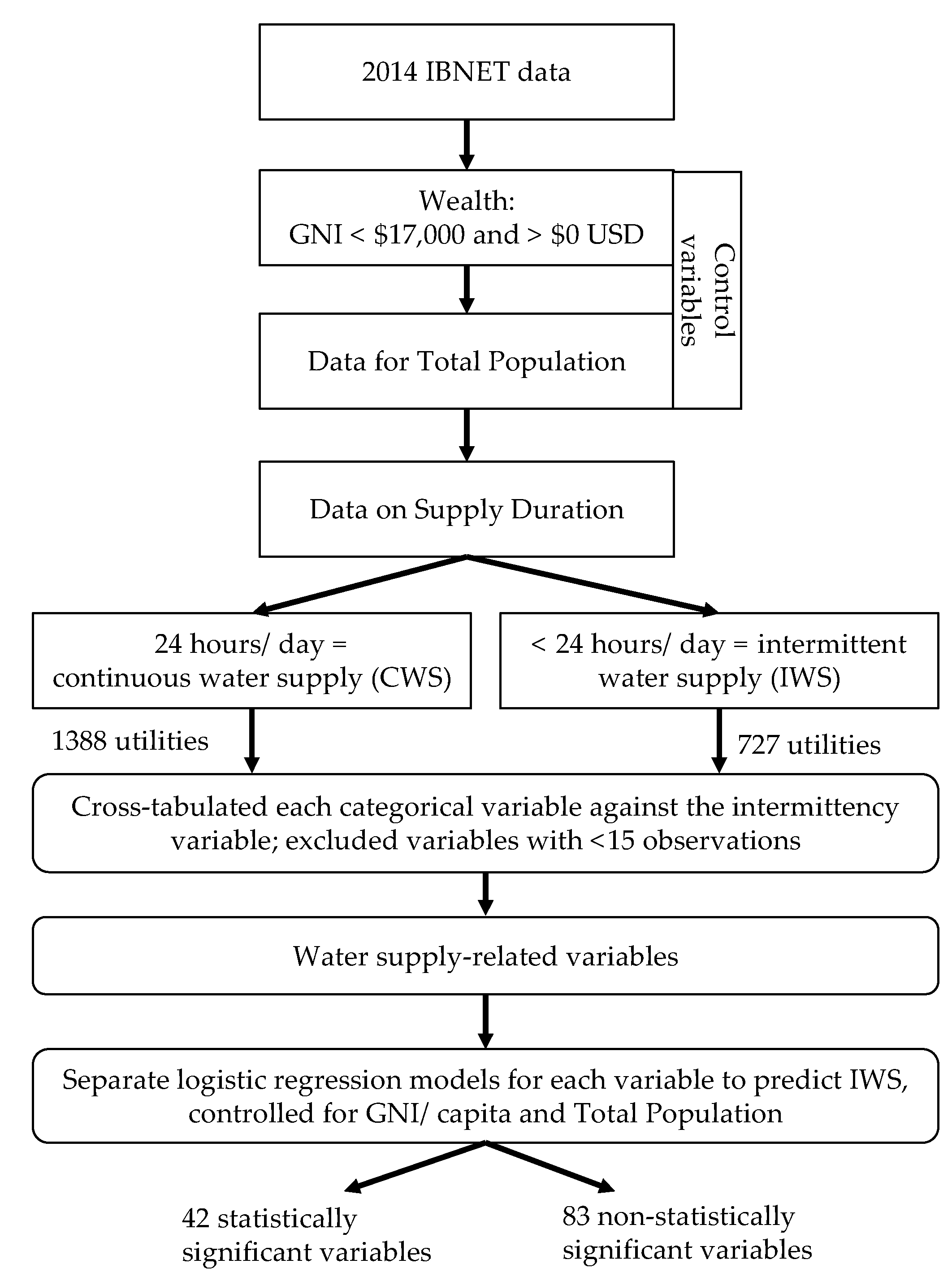
The data used in this analysis were obtained from IBNET in May 2017. As described below, the final dataset represents 2115 utilities from 46 countries (Figure 1 and Figure 2). All IBNET variables that describe water services were included in this analysis. Variables that considered just wastewater services or that combined measures for water and wastewater were dropped, as many utilities do not provide wastewater services, and as the literature does not suggest that the performance of the wastewater system would be a useful predictor for the water infrastructure of interest to this analysis. Utility data from 2014 was selected for this analysis because it had a significantly larger number of data points than either 2015 or 2016. After cleaning the dataset, we coded utilities as having either intermittent or continuous supply based on the number of hours per day of supply they reported in the IBNET data. Utilities with 24-h supply were coded as continuous, utilities that did not respond to this question were dropped from the analysis, and all others were coded as intermittent. Notably, these data reflect only the daily hours of supply and not whether there are multiple days between supply, or what percentage of the infrastructure network or population receives intermittent supply.

After creating these categories, we noted that none of the utilities in the wealthiest contexts (as measured by the gross national income (GNI) per capita variable provided by IBNET) reported intermittent supply. Specifically, in the cleaned 2014 IBNET dataset, all 163 utilities in contexts with per capita GNI above $17,000 USD reported continuous supply. As such, and given our particular interest in low and middle income countries (LMIC), we limited our analysis to those utilities in contexts with per capita GNI less than $17,000 USD, and also included per capita GNI as a control variable in the analysis. Two utilities reported a per capita GNI of $0 USD; we excluded these from the analysis to maintain data consistency. We also wanted to control for the urban vs. rural nature of the service area. While utilities enter an urban/rural classification for themselves in the IBNET data, only 11 utilities reported being entirely rural in the 2014 dataset. In addition, we felt the definition utilities were using to classify themselves as urban or rural likely varied from utility to utility. As such, we instead control for an urban/rural proxy using the IBNET variable 30, which measures the “total population under notional responsibility of the utility for water supply, irrespective of whether they receive service”. In other words, this control variable is indicative of the scale of population living in the context the utility operates in. This results in a cleaned dataset of 2115 utilities, of which 1388 report continuous supply and 727 report intermittent supply (Figure 2).

Next, we cross-tabulated each categorical variable against the created binary intermittency variable, and excluded all categories that did not have at least 15 observations for each combination. When necessary, the exchange rate listed in the IBNET data was used to convert financial variables to USD. Finally, we ran separate multiple logistic regression models using each water-supply related variable in the IBNET data to predict intermittency in supply, while controlling for GNI/capita and the urban/rural nature of the service area as described above [26]. All regression models permit the discovery of relationships between a predictor and explanatory variables. For example, in the engineering literature, regression has been used to explore locally appropriate structures of public private partnerships for water and sewerage infrastructure [27] or global variations in water infrastructure technology choice [28]. Here, we model a categorical dependent variable with outcomes that have no natural ordering; thus, we use a multiple logit model, which is generalized as below.

For a set of p independent variables x’ = (x₁, x₂, x₃…x_p), the probability that the outcome is present is given by P(Y = 1|x) = π(x). Then, the logit of the multiple logistic regression model is:

$$\mathrm{g}\left(\mathrm{x}\right)=\ln \frac{\pi \left(x\right)}{1-\pi \left(x\right)}={\mathsf{\beta }}_0+{\mathsf{\beta }}_1{\mathrm{x}}_1+{\mathsf{\beta }}_2{\mathrm{x}}_2+\dots +{\mathsf{\beta }}_p{\mathrm{x}}_p,$$

where β_0–p are variable coefficients and

$$\pi \left(\mathrm{x}\right)=\frac{{\mathrm{e}}^{\mathrm{g}\left(\mathrm{x}\right)}}{1+{\mathrm{e}}^{\mathrm{g}\left(\mathrm{x}\right)}}$$

Each model run represents a different number of utility observations, as different numbers of utilities answered each question in the IBNET database. This number is listed in the results table for each model run. The Table S1 includes the results for all model runs. As space does not permit us to discuss all 125 model runs,

Table 1. Main themes identified through analysis of variables with their definition and highlighted findings.

Results Section	Theme	Definition and Example Variables	Highlighted Findings Utilities were Correlated with IWS
3.1	Physical infrastructure system scale	Overall size of the infrastructure system (e.g., water volumes, distribution network)	Producing less water No correlation with variables related to network density, length
3.2	Coverage	Numbers or percent of people	Serving lower percentages of the population
3.3	Water consumer type	Provision of water by customer group (e.g., residential, commercial)	Selling and billing less water volumes Generating more revenue from residential consumers and less from commercial/industrial consumers
3.4	Public water points	Presence and use of shared or public water points	Serving more people through public water points
3.5	Financial	Financial metrics, such as operating costs and revenues	With lower operating cost coverage and revenues No correlation with many other financial metrics
3.6	Non-revenue water and metering	Accounting and losses of water in the distribution system	Lower numbers, rates, and billings related to metering No correlation with non-revenue water

,

Table 2. A selection of variables related to physical infrastructure system and their relationship to intermittent (<24 h) vs. continuous (24 h) supply. Includes variable number and names as used in the International Benchmarking Network (IBNET) database (ib-net.org), number of observations (n), the p value (p), the relative risk ratio (RR), and an interpretation of the results.

IBNET Variable	IBNET Variable Name	n	p	RR	What is Associated with Intermittent Supply?
Raw data
40	Population Served-Water	2108	0.002 *	<1	Lower Population Served/Number of Connections
41	Number of Water Connections	2005	0.009 *	<1
54	Length of Water Distribution Network (km)	2019	0.137	-	-
-	Capacity (million m3/year)
42	Design Capacity of Intakes	579	0.039 *	>1	Higher Design Capacity
55	Volume of Water Produced	2095	0.000 **	<1	Lower Volume of Water Produced
Indicators
1 × 4	Network Density (con/km)	1913	0.173	-	-
-	Water Production
3.1	L/person/day	2093	0.003 *	<1	Lower Water Production
3.2	m3/connection/month	1985	0.59	-	-
	Consumption (L/person/day)
4.7	Residential	1759	0.000 **	<1	Lower Residential Consumption/Capacity Utilization
30.1	Capacity Utilization (m3 produced/intake design capacity) (%)	464	0.02 *	<1

Notes: Reference category for equation is Continuous Supply. Controls for GNI/capita and nominal service population. Includes only utilities with reported GNI/capita less than $17,001 USD. * p < 0.05; ** p < 0.000.

,

Table 3. A selection of variables related to coverage, water consumer type, and public water points and their relationship to intermittent (<24 h) vs. continuous (24 h) supply. Includes variable number and names as used in the IBNET database (ib-net.org), number of observations (n), the p value (p), the relative risk ratio (RR), and an interpretation of the results.

IBNET Variable	IBNET Variable Name	n	p	RR	What is Associated with Intermittent Supply?
Raw Data
40b	Population Served-Public Water Points	559	0.01 *	>1	Higher Population Served-Public Water Points
43	Number of Public Water Points	434	0.439	-	-
-	Volume of Water Sold (million m3/year)
-	Total Customers				Lower Volume of Water Sold/ Sold to Residential Customers/ Direct Supplies
59	Residential	2099	0.000 **	<1
59a	Total	1752	0.007 *	<1
59a1	through Direct Supplies	666	0.002 *	<1
59a2	through Public Water Points	495	0.17	-	-
59b	Industrial/Commercial	1223	0.05 *	<1	Lower Volume of Water Sold to Industrial, Commercial/Institutions, Others
59c	Institutions/Others	686	0.001 *	<1
59d	Treated in Bulk	469	0.099	-	-
	Total Water Billings (USD)
90e	Residential	679	0.000 **	<1	Lower Total Water Billings to Residential/Industrial, Commercial/Institutions, Other
90f	Industrial/Commercial	673	0.000 **	<1
90g	Institutions/Other	627	0.011 *	< 1
90h	Bulk Treated Supplies	383	0.168	-	-
Indicators
-	Water Coverage (%)
1.1	Total	2104	0.001 *	<1	Lower Water Coverage/Household Connections
1.2	Household Connections	738	0.000 **	<1
1.3	Public Water Points	534	0.012 *	>1	Higher Water Coverage—Public Water Points
-	Consumption (%)
4.3	Residential	1756	0.305	-	-
4.4	Industrial/Commercial	1411	0.000 **	>1	Higher Industrial, Commercial Consumption
4.5	Institutions and Others	681	0.017 *	<1	Lower Consumption by Institutions, Others
4.6	Bulk Treated Supply	466	0.207	-	-
4.9	Public Water Points	262	0.376	-	-
-	Water Revenue (% total water revenue)
18.6	Residential	666	0.015 *	>1	Higher Water Revenue—Residential
18.7	Industrial/Commercial	656	0.000 **	<1	Lower Water Revenue—Industrial, Commercial
18.8	Institutions/Other	612	0.454	-	-
18.9	Bulk Treated Supply	376	0.829	-	-
21.2	Ratio of Industrial to Residential Tariff—Water (ratio)	606	0.777	-	-
24.1	Operating Cost Coverage (Operational revenues/costs)	1998	0.000**	<1	Lower Operating Cost Coverage

Notes: Reference category for equation is Continuous Supply. Controls for GNI/capita and nominal service population. Includes only utilities with reported GNI/capita less than $17,001 USD. * p < 0.05; ** p < 0.000.

,

Table 4. Relationship between intermittency and customer type by measures of volume of water sold, consumption and revenue as a percent of the total, and water billings (summarized from Table 3).

Customer Type	Volume Sold (59–59d)	Consumption (% total) (4.3–4.6)	Revenue (% total) (18.6–18.9)	Billings (90e–90h)
Residential	Lower	-	Higher	Lower
Commercial/Industrial	Lower	Higher	Lower	Lower
Institutional/Other	Lower	Lower	-	Lower
Bulk	-	-	-	-
Total	Lower	-	-	N/A a

^a not available (N/A): variable for total billings for only water (i.e., excluding wastewater) unavailable.

and

Table 5. A selection of variables related to finances, non-revenue water, and metering, and their relationship to intermittent (<24 h) vs. continuous (24 h) supply. Includes variable number and names as used in the IBNET database (ib-net.org), number of observations (n), the p value (p), the relative risk ratio (RR), and an interpretation of the results.

IBNET Variable	IBNET Variable Name	n	p	RR	What is Associated with Intermittent Supply?
Raw Data
-	Expenses for Water (USD/year)
94a	Total Operational Expenses	1813	0.111	-	-
97	Electrical Energy	1929	0.035 *	<1	Lower Electrical Energy/Repair and Maintenance Costs
98	Repair and Maintenance	625	0.003 *	<1
-	Metering for Water
53	Number of Connections with Operating Meter	1987	0.043 *	<1	Lower Number of Water Connections with an Operating Meter/Volume of Water Consumed Metered
58	Volume of Consumed Metered (million m3/year)	1734	0.024 *	<1
Indicators
11.3	Unit Operational Cost-Water Only (USD/m3 sold)	1761	0.41	-	-
13.2	Electrical Energy Costs as Percent of Operational Costs (%)	1886	0.652	-	-
19.1	Total Revenues per Service Population (% GNI per capita)	2056	0.016 *	<1	Lower Total Revenues per Service Population/GNI
30.5	Average Cost of Each Repair (USD/repair)	159	0.523	-	-
-	Non-Revenue Water
6.1	%	2090	0.377	-	-
6.2	m3/km/day	1993	0.075	-	-
6.3	m3/connection/day	1982	0.497	-	-
-	Metering for Water (%)
7.1	Level	1957	0.000 **	<1	Lower Metering Level/Water Sold that is Metered
8.1	Water Sold that is Metered	1725	0.000 **	<1

Notes: Reference category for equation is Continuous Supply. Controls for GNI/capita and nominal service population. Includes only utilities with reported GNI/capita less than $17,001 USD. * p < 0.05; ** p < 0.000.

include results that are discussed here. The STATA 14 software package was used for this analysis.

Variables that are statistically significant predictors of intermittent water supply are indicated in Table 2, Table 3 and Table 5, and the Table S1 by a starred p value. For this exploratory work, we indicate two thresholds for statistical significance. The first (indicated by a single star) identifies variables that are statistically significant at the p < 0.05 level. This significance level means that there is a 5% likelihood that the observed relationships are due to chance. As we conducted 125 tests on the same dataset, we would expect to see about seven falsely significant results (Type 1 error). One conservative way to handle this issue of multiple comparisons is the Bonferroni correction [29]. This divides the required significance threshold value by the number of statistical tests to determine a stricter criterion for significance (here, 0.05/125 = 0.0004). This correction gives us our second threshold for significance, where any variable with significance level lower than 0.000 is flagged with two stars in Table 2, Table 3 and Table 5 and the Table S1. This type of a correction reduces Type I error at the cost of increased Type II error—in other words, the chance of missing something important increases. Given the exploratory nature of this analysis, we claim that any result with a p value below 0.05 is worth further investigation, with the caveat that we are most confident in the significance of variables with a p value below 0.000.

It is also worth noting that Table 2, Table 3 and Table 5 and the Table S1 indicate only the directionality of relationships rather than exact relative risk ratios. This is because the values of relative risk ratios are sensitive to the units of the predictors, which cannot be standardized in this analysis (for example, it is not possible to standardize the units of Number of Towns Served with Water and Electricity Consumption-Water).

A limitation of this analysis is that the IBNET data is self-reported by utilities. In addition, the IBNET data tends to be more comprehensive for more highly resourced utilities. These two factors may bias the reported data towards better utility performance. In addition, this analysis dichotomizes utilities as having either intermittent or continuous supply. However, we might reasonably expect that a utility that reports a water supply 23.9 h out of the day to be different than one that only provides a few hours’ supply each day. Future work should explore these differences. It is also worth emphasizing that the associations described here do not prove causation; future research with different designs is needed to explore these results. In addition, this statistical analysis should be repeated in the future should more complete data become available. Finally, the standardization that is the strength of the IBNET data also results in simplified measures that may not always adequately represent local complexities. This is a limitation common to nearly any large-n data collection effort. Future qualitative research can address this limitation by exploring key factors in detailed, case study research. Still, the present exploratory analysis is a valuable beginning, as it identifies aggregate trends that have strong potential for wide, generalized application.

3. Results

Space does not permit us to discuss each of the 125 results, or even all of the 42 variables that meet at least one of our significance thresholds. As such, we have selected topics and sets of variables for discussion that contribute to conversations in the literature treating intermittent water supply (Table 2). The IBNET variables selected for discussion and logistical regression results are presented in Table 3, Table 4 and Table 5, and referenced throughout the discussion by the IBNET variable number (other results are provided in the Table S1). In an example of results from Table 2, a lower value of IBET Variable 40 (Population Served-Water) is associated with intermittent supply at a statistically significant level (p = 0.002). We include both the raw data and the IBNET-calculated indicators as variables in our analysis.

3.1. Physical Infrastructure System Scale

Many of the variables in the IBNET data describe the physical infrastructure system scale. For example, the population served (40), the number of water connections (41), the design capacity of water intakes (42), length of the distribution network (54), network density (1 × 4), and volume of water produced (55, 3.1, 3.2) all directly describe the physical scale of the system (Table 2). The data show that some—but not all—of these physical descriptors are significant predictors of intermittent water supply. As such, these relationships may provide insights for resilient water infrastructure design, monitoring, and evaluation.

For example, lower water production per person (3.1) and lower raw volume of water produced by the utility (55) are significant predictors of intermittency (Table 2). In some instances, this result could be due to water rationing, shrinking demands from water use efficiency gains, or organizational efficiencies of scale. Regardless, utilities in our dataset that produce less water are more likely to have intermittent supply than utilities that produce more water.

In contrast to the above metrics, water production per connection (3.2) is not a statistically significant predictor of intermittency (Table 2). We explain this by noting that both the number of households in low- and middle-income countries (LMICs) using a single connection and the flow rate of each connection can vary significantly, and that connections are thereby a weaker indicator of water demand than population. In a supply-constrained intermittent system, a limited amount of water is then shared by a larger number of people, reducing per-person consumption [5]. In this sense, connections are a constraint between the production and consumption of water. We expect that this constraint would influence households more than other customer types, because the majority of the raw count of connections (41) go to households rather than the larger commercial customers. Indeed, the data show that both a lower count of water connections (41) and lower residential consumption in liters/capita/day (4.7) correlate with a higher likelihood of intermittent supply (Table 2).

In a related metric, lower Capacity Utilization (30.1), which measures the ratio of how much water is actually produced compared to the intake design capacity, is also correlated with a higher likelihood of intermittent supply (Table 2). This normalization provides the counterintuitive insight that systems that operate near full volume capacity are more likely to provide continuous supply than are systems with excess volume capacity. The significance of this indicator is not only due to the relationships just described for the numerator (water production, 3.1); the denominator (raw water intake design capacity, 42) is also statistically significant. Counterintuitively, higher raw water intake design capacities mean intermittent water supply is more likely. In some cases, this may be because production limitations such as treatment process capacities or limits on energy availability to pump water prevent water from being delivered to the network despite intake capacity, because physical water shortages prevent systems from taking in what they were designed to take in, or because seasonal variability in water availability and demand cause difficulties in infrastructure sizing.

Network density (1 × 4) and the raw distribution system length (54) are also not significant predictors of intermittent water supply (Table 2). This suggests that it is not the physical design that limits water infrastructure performance, but rather that performance issues occur depending on usage or operational factors. Kleemeier found in rural Malawi that smaller water systems performed better than the larger systems, noting that it is easier to locate problems in small systems due to their size, simplicity, and ease of operator travel within the system [30]. However, in the literature, findings on the connection between utility size and performance is conflicted and evidence of an association between customer density and utility performance is scarce, particularly in low and middle income countries. One study within a single country (Italy) found a positive correlation between density and cost efficiency [31].

In sum, and with the caveat regarding intake design capacity, intermittent water supply is more likely when there is less water available from the water infrastructure. For households, this is true regardless of whether the availability constraint is due to production or access limitations. More discussion of the relationship between consumer types, non-revenue, and intermittency follows. In addition, most scale metrics that are normalized based on infrastructure parameters (such as length, density, connection count, etc.) rather than people (population) are not significant predictors of intermittent water supply.

3.2. Coverage

Three variables in the IBNET data describe water service coverage (Indicators 1.1, 1.2, and 1.3) (Table 3). Overall water coverage (1.1) is the “population with access to water services (either with direct service connection or within reach of a public water point) as a percentage of the total population under utility’s nominal responsibility” [32]. Coverage is a key development indicator; for example, it operationalizes the Sustainable Development Goals for water and sanitation [33]. However, coverage metrics are limited—for example, they indicate potential access but not quality or equity of service.

For this aggregate coverage metric, lower water coverage is a strongly significant predictor of intermittent water supply (1.1, p = 0.001) (Table 3). Said another way, the data show that utilities that are able to serve a higher percentage of the population within their designated service area are also better able to provide continuous supply. While the present research design cannot determine why we observe this relationship in the data nor yet a direction of causality, one possible explanation is rapid population growth that outpaces utility expansion. The other two coverage variables (1.2 and 1.3) provide some insight to this relationship by splitting this aggregate figure into coverage via household connections and public water points (PWP) (Table 3). The observed relationships between intermittency and these two measures are statistically significant and directionally opposed, with intermittency predicted by lower rates of household connections and higher rates of coverage via public water points. This split, and its implications for the relationship between coverage and intermittency, is discussed in more detail below.

3.3. Water Consumer Type

Water utilities provide water to different types of consumers, which in the IBNET database are separated four types: Residential, commercial/industrial, institutions, and bulk water. The variables included in the IBNET database compare the volume of water consumed by and sold to these different groups and associated billings and revenues; the statistically observed relationships between these variables are listed in Table 3 and further summarized in Table 4.

As discussed previously, lower volumes of water sold (59a–c), and correspondingly lower total water billings (90e–90g) tend to be associated with intermittency (Table 3 and Table 4). These trends are statistically significant for all consumer types except bulk water customers. However, these consistent relationships are not seen across either percent consumption or percent revenue by consumer type (4.3–4.6; 18.6–18.9) (Table 3 and Table 4).

For example, both higher percent revenue from residential consumers (18.6) and lower percent revenue from commercial/industrial consumers (18.7) are associated with increased intermittency in water supply (Table 3). Although these groups are often charged different rates, the ratio of industrial to residential tariffs for water (21.2) was not significantly associated with intermittency (Table 3). Taken alone, these findings suggest that utilities interested in reducing intermittency could target revenue generation from commercial/industrial consumers rather than residential consumers. However, this interpretation is complicated by the relationships observed in the data describing consumption by consumer type. Higher volume of commercial/industrial consumption (59b) is associated with increased intermittency, while residential consumption (59a2) does not show a significant relationship with intermittency (Table 3 and Table 4). It is worth noting that not all water consumed is paid for, and that, especially in the case of residential customers’ consumption, data may be based on estimates rather than metered values.

Together, these results suggest that both demand management and/or revenue generation from commercial/industrial customers may be key leverage points for reducing intermittent water supply. Localized research is needed to build typologies of mechanisms behind these statistically observed relationships. For example, in some contexts, geographically or temporally concentrated demands from larger commercial/industrial customers may overwhelm system capacity and cause local intermittency, or may lead utilities to prioritize supply to these consumers. In other contexts, non-payment of the larger bills from this customer type may disproportionately impact financial resiliency and thereby contribute to intermittent supply. Alternatively, residential customers typically have smaller pipes, smaller connections, and simply consume less per connection than do the larger industrial/commercial customers. As such, it is logistically (if not always politically) easier for utilities to maintain, bill, and generate revenue from the larger industrial/commercial customers. Following this line of logic suggests that when this customer type is not present, utilities have a higher logistical challenge in achieving revenue generation that would fund continuous supply. A report in the US found that water systems serving smaller populations, which also tended to have limited finances, had more of their revenue coming from residential customers than larger utilities, which relied more on revenue from non-residential customers. It was also noted that non-residential customers in small water systems are often small businesses, which have less water use than large, commercial/industrial customers [34]. Given these and other competing explanations for the statistically observed relationships, future research is needed to explore these findings.

3.4. Public Water Points

Several IBNET variables relate to the presence and use of shared or public water points (PWP) (although we note that alternative sources such as private water vendors or groundwater supplies are not included in the dataset). These include the population served by PWPs (40b, 1.3), the total number of PWPs in the system (43), the volume of water sold to residential customers through PWPs (59a2), and the residential consumption from PWPs in liters/capita/day (4.9) (Table 3). The nature of PWPs may vary across utilities: PWPs can be free of charge, or may be set up as a kiosk where water is sold by the jerry can. In addition, the source of the water for the PWPs could be the piped system that also supplies household connections or non-networked sources such as a hand pump connected to wells that were installed, maintained, or operated by the utility.

Of these, the only variables that are statistically significant predictors of intermittent supply related to the type of connection used by the population: as the number of people served by PWPs (40b) or the percentage of the population served by PWPs (1.3) increased, the supply was more likely to be intermittent. The corollary was also true: The lower percentage of people served by household connections, the more intermittent the supply (1.2) (Table 3).

These results seem to support prominent efforts to convert intermittent supply to continuous water supply in India. Several of these efforts have included closing what were previously free PWPs from both the distribution network and from alternative water sources [3,35,36]. One assumption behind these policies is that water provided for free is not used efficiently, allowing people to draw more water than their demand or allowing taps to flowing open, leading to higher network demand and reduced cost recovery [37]. However, in contrast to this discourse, the data show that the volume of water sold (but per IBNET definitions not necessarily paid for) through PWPs (59a2) is not significantly associated with continuity. A second assumption embedded in policies that close PWPs is the idea that in order to achieve a sustainable water supply network, water needs to be accounted and paid for to achieve cost recovery (the epistemology of water infrastructure as a service [38]). Indeed, in the IBNET data, lower Operating Cost Coverage (24.1) is associated with intermittency (Table 3). However, this discourse is problematized by Indicator 18.6, which shows that higher percentage of total revenues coming from residential customers are actually statistically significant predictor of intermittency. Additionally, per capita water use from PWPs (4.9) was not significantly associated with continuity, further suggesting that PWPs may not have higher per-capita use (Table 3). In an intermittent supply with short supply hours, households drawing water from shared taps have been observed to consume significantly less water per capita than households with private taps [5]. Future work on financial management of public water points could assist in better understanding this connection between continuity and PWPs. Additionally, this issue links closely to our earlier discussion of customer types.

While the above policy logic posits PWPs as a potential cause of intermittency, they may also be a reaction to intermittency. Such points may be installed by utilities during times of water supply shortage (i.e., the more unreliable the piped water supply, the more need for alternative water supplies). On the other hand, in the absence of adequate public provision of water supply, households incur costs associated with obtaining and maintaining a reliable, high-quality water supply (e.g., purchasing or spending time collecting water from alternative sources) [8,39,40]. Therefore, efforts to improve public provision of water through a networked supply aim to shift the costs from household expenditures toward their water tariff [8,36]. Finally, kiosks where people may purchase water are often installed where the network does not reach communities or where responsibility for management and payment to users shifts from the utility to user associations [41]. As such, common use of PWPs may often be indicative of a system with low piped coverage. As low water coverage (1.1) is also statistically predictive of intermittency, the relationships between these variables should be explored in future research.

3.5. Financial

The analysis presented here controls for GNI per capita. This means that the observed relationships are not just a function of economic capacity, though we cannot rule out the influence of economic inequality with this dataset. Still, the data show some that financial metrics are significant predictors of intermittency (Table 3). For example, utilities with lower operating cost coverage (24.1) are more likely to provide intermittent water supply. Similarly, utilities with lower total revenues expressed as a percentage of GNI (19.1) are more likely to provide intermittent water supply (Table 5). These data show that utilities that have more resources are better able to provide water; accordingly, intermittent supply is also predicted by lower total electrical energy costs and by repair and maintenance costs (97, 98). However, total operational expenses (94a) is not a significant predictor of intermittency (Table 5). This suggests that resources must be both available and spent on the right things in order to produce continuous water supply. Still, the large number of financial metrics that do not have a significant relationship with intermittent supply suggest that these metrics may not be able to adequately reflect individual utility context. For example, and as noted above, the data show that utilities that spend more on electricity and repairs provide better service. However, electrical energy costs as a percentage of operational costs (13.2) or even the more encompassing unit operational cost of water (11.3) are not significant predictors of intermittency. Similarly, while repair and maintenance expenditures (98) is significant, the average cost of each repair (30.5) is not (Table 5).

While future research is needed to confirm this interpretation, we suggest these mixed results are because the cost of providing water necessarily varies depending on context. Unfortunately, many of the existing metrics do not capture these variations, and this means that even intuitively appealing indicators such as the unit cost of water (11.3) ignore important contextual normalizers (Table 5). Without these, we simply cannot determine whether (for example) higher unit costs are due to waste or necessity; the absence of observed trends in the data suggests that these explanations are competing rather than dominant in our dataset. More universally true (and thereby emerging as statistically significant) are the ideas that water utilities must spend money on items such as repairs and electricity, and that they need to generate sufficient revenue to cover these costs. This emphasis on sufficient resources vs. inefficiencies leads to our next discussion theme of non-revenue water.

3.6. Non-Revenue Water and Metering

Non-revenue water (NRW) is a metric that represents water delivered through the distribution system that is not paid for. NRW includes physical losses (water lost through leaks, storage tank overflows), commercial losses (e.g., inaccuracies in meters, theft), and unbilled authorized consumption (water provided free of charge, such as at PWPs, for firefighting, or by authorized government agencies) [42,43]. Three variables in the IBNET database present NRW as a percent of water supplied to the network, m³/km/day, or m³/connection/day (6.1–6.3, Table 5). Surprisingly, none of these variables were significantly associated with continuity, despite the ongoing focus on reducing NRW in order to improve utility performance [42].

However, NRW combines the three types of losses (physical, commercial, and unbilled authorized consumption). It has been posited that physical losses may be one of the most important components of losses in intermittent supply, with estimates of 50 or 60% physical losses not uncommon [5,42,43,44]. Importantly, physical losses are affected by several interconnected features of intermittent supply [44,45]. First, physical loss measurements do not account for fewer hours of supply: Losses are measured as the total water supplied (or paid for) divided by the total water provided to the network. However, since water in an intermittent supply is provided for only short periods of time, physical losses would be much greater if water were provided for the full 24 h per day. Therefore, Frauendorfer and Liemberger [42] put forward that to make a fair comparison, losses in intermittent supplies should be measured as a fraction of the water that would be supplied if it were on for 24 h of the day. Secondly, physical water losses are pressure-dependent (more water flows out of an orifice at higher pressures). Since intermittent supplies are supply-driven systems, pressures tend to be very low [2,46]. These low-pressure networks are therefore expected to have less physical losses compared to higher pressure networks. Together, these observations may explain why the data do not show a significant association between intermittent supply and NRW.

A second component of NRW is commercial losses, which depends on metering. Notably, metering and intermittency are correlated in our dataset: The number of connections with an operating meter (53), the volume of water consumed that was metered (58), the percent of connections that are metered (7.1), and the percent of water sold that was metered (8.1) are all inversely associated with intermittency (lower metering metrics associated with more intermittency) (Table 5). Ongoing initiatives to shift service from intermittent to continuous supply include installation of meters to account for losses, regulate water use (e.g., through the introduction of increasing block rate tariffs), and increase cost-recovery [47]. Therefore, the association between lower metering and lower hours of supply matches policy prescriptions for transitioning from intermittent to continuous supply, although this relationship may have confounded potential relationships between NRW and intermittency.

4. Discussion

The objective of this analysis was to explore correlations between utility benchmarking data and intermittent supply, with the goal of confirming important and identifying new associations to highlight opportunities for future research that elucidates the causes of—and ultimately, solutions to—intermittent supply. In the set of 125 variables analyzed in the IBET database, 42 variables were statistically significant; however, even those which were not statistically significant offer interesting insights. For example, we found that intermittent water supply was associated with utilities that had less water available from the water infrastructure, were only able to serve a lower percentage of the population in their service area, were more dependent on public water points than residential connections for providing access, and had lower rates of metering. Furthermore, we also identified new insights into associations with intermittency or usefulness of indicators in this context: For example, the measurement of non-revenue water may be confounded in intermittent supply [45]; costs, since they are highly context specific, need to be more carefully analyzed to understand what utilities should spent their money on to achieve CWS; and commercial and industrial customers may be a leverage points for reducing intermittent water supply. Our study design and available data allowed us to explore only correlations, not causation; many of these identified relationships are likely both causes and consequences of intermittent supply. Throughout this analysis, we identified opportunities for future research that could be followed up with through a variety of study designs; localized case studies that provide context-specific knowledge have been conducted and continue to provide value [48], while designs that track transitions to and from IWS to CSW or that aggregate results across contexts should be explored.

This analysis shows both the potential for and limitations of standardized utility performance indicators. The ability to analyze large numbers of utilities has the potential to bring new insights to the policy and practice of water management; for example, the IBNET data we discuss here problematizes influential discourses regarding public water points and NRW. Still, a key limitation of this kind of analysis is that we cannot discover the mechanisms that are behind the empirically observed relationships; this must be left for future research that uses different research designs. This may be particularly important for civil infrastructure systems such as water supply networks, which are heavily influenced by both technical and social factors (for example, NRW is influenced by both operating pressure and also commercial losses such as theft). As such, the data highlight the importance of demand and usage predictability. For IWS in particular, this analysis also highlights the need for characterizing typologies of intermittent supply that can be more tightly linked to solutions.

As is typical for civil infrastructure, both local and generalizable factors must be considered in order to achieve good infrastructure outcomes [49]. The relationships discussed here suggest, for example, that (for IWS) the best global indicators for water infrastructure are baselined on population and demand rather than by physical infrastructure scale. Similarly, if global indicators are to be broadly relevant for comparison across contexts they must include contextualized reference points. Much as cross-national economics convert currencies to a common baseline, infrastructure metrics must also be grounded in the local context. For water infrastructure, this could include the source of water (e.g., groundwater vs. surface water), levels of treatment (e.g., primary, secondary, tertiary), energy sources (e.g., diesel generator vs. grid electricity), resource costs (e.g., raw water, labor, energy), geographic challenges (e.g., small island nations vs. large, landlocked nations), climate (e.g., water scarcity and demands), etc. This kind of contextual knowledge, which should be feasible to collect, would enable the creation of targeted indicators baselined for cross-context comparisons, such as expected costs of providing services or of the expected relative difficulty of achieving desired infrastructure outcomes.

References

- Bivins, A.W.; Sumner, T.; Kumpel, E.; Howard, G.; Cumming, O.; Ross, I.; Nelson, K.; Brown, J. Estimating Infection Risks and the Global Burden of Diarrheal Disease Attributable to Intermittent Water Supply Using QMRA. Environ. Sci. Technol. 2017, 51, 7542–7551. [Google Scholar] [CrossRef] [PubMed]
- Kumpel, E.; Nelson, K.L. Intermittent Water Supply: Prevalence, Practice, and Microbial Water Quality. Environ. Sci. Technol. 2016, 50. [Google Scholar] [CrossRef] [PubMed]
- Sangameswaran, P.; Madhav, R.; D’Rozario, C. 24/7, “Privatisation” and water reform: insights from Hubli-Dharwad. Econ. Polit. Wkly. 2008, 43, 60–67. [Google Scholar]
- Thompson, J.; Porras, I.T.; Tumwine, J.K.; Mujwahuzi, M.R.; Katui-Katua, M.; Johnstone, N.; Wood, L. Drawers of Water II: 30 Years of Change in Domestic Water Use and Environmental Health in East Africa; International Institute for Environment and Development: London, UK, 2001. [Google Scholar]
- Kumpel, E.; Woelfle-Erskine, C.; Ray, I.; Nelson, K.L. Measuring household consumption and waste in unmetered, intermittent piped water systems: Water Use in Intermittent Piped Systems. Water Resour. Res. 2017. [Google Scholar] [CrossRef]
- Kumpel, E.; Nelson, K.L. Comparing Microbial Water Quality in an Intermittent and Continuous Piped Water Supply. Water Res. 2013, 47, 5176–5188. [Google Scholar] [CrossRef] [PubMed]
- Ercumen, A.; Arnold, B.F.; Kumpel, E.; Burt, Z.; Ray, I.; Nelson, K.; Colford, J.M., Jr. Upgrading a Piped Water Supply from Intermittent to Continuous Delivery and Association with Waterborne Illness: A Matched Cohort Study in Urban India. PLOS Med. 2015, 12, e1001892. [Google Scholar] [CrossRef] [PubMed]
- Zerah, M.H. How to assess the quality dimension of urban infrastructure: The case of water supply in Delhi. Cities 1998, 15, 285–290. [Google Scholar] [CrossRef]
- Pattanayak, S.K.; Yang, J.-C.; Whittington, D.; Bal Kumar, K.C. Coping with unreliable public water supplies: Averting expenditures by households in Kathmandu, Nepal. Water Resour. Res. 2005, 41. [Google Scholar] [CrossRef] [Green Version]
- Sashikumar, N.; Mohankumar, M.S.; Sridharan, K. Modelling an Intermittent Water Supply. World Water Environ. Resour. Congr. 2003, 118, 261. [Google Scholar]
- Matsinhe, N.P.; Juízo, D.L.; Persson, K.M. The Effects of Intermittent Supply and Household Storage in the Quality of Drinking Water in Maputo. VATTEN J. Water Manag. Res. 2014, 70, 51–60. [Google Scholar]
- Christodoulou, S.; Agathokleous, A. A study on the effects of intermittent water supply on the vulnerability of urban water distribution networks. Water Sci. Technol. Water Supply 2012, 12, 523–530. [Google Scholar] [CrossRef]
- Misra, K.; Malhotra, G. Water management: the obscurity of demand and supply in Delhi, India. Manag. Environ. Qual. Int. J. 2012, 23, 23–35. [Google Scholar] [CrossRef]
- Faust, K.M.; Abraham, D.M.; McElmurry, S.P. Water and wastewater infrastructure management in shrinking cities. Public Work. Manag. Policy 2016, 21, 128–156. [Google Scholar] [CrossRef]
- Faust, K.M.; Abraham, D.M.; DeLaurentis, D. Coupled Human and Water Infrastructure Systems Sector Interdependencies: Framework Evaluating the Impact of Cities Experiencing Urban Decline. J. Water Resour. Plan. Manag. 2017, 143, 4017043. [Google Scholar] [CrossRef]
- Galiani, S.; Gertler, P.; Schargrosky, E. Water for life: the impact of the privatization of water services on child mortality. J. Polit. Econ. 2005, 11, 83–120. [Google Scholar] [CrossRef]
- Bhanwar, S.; Ramasubban, R.; Bhatia, R.; Briscoe, J.; Griffin, C.C.; Kim, C. Rural water supply in Kerala, India: how to emerge from a low-level equilibrium trap. Water Resour. Res. 1993, 29, 1931–1942. [Google Scholar]
- Tamayo, G.; Barrantes, R.; Conterno, E. Reform efforts and low-level equilibrium in the Peruvian water sector. In Spilled Water: Institutional Commitment in the Provision of Water Services; Inter-American Development Bank: Washington, DC, USA, 1999; pp. 89–134. [Google Scholar]
- Galaitsi, S.E.; Russell, R.; Bishara, A.; Durant, J.L.; Bogle, J.; Huber-Lee, A. Intermittent Domestic Water Supply: A Critical Review and Analysis of Causal-Consequential Pathways. Water 2016, 8, 274. [Google Scholar] [CrossRef]
- Totsuka, N.; Trifunovic, N.; Vairavamoorthy, K. Intermittent urban water supply under water starving situations. In 30th WEDC International Conference; WEDC: Vientiane, Lao PDR, 2004. [Google Scholar]
- Walters, J.P.; Javernick-Will, A.N. Long-Term Functionality of Rural Water Services in Developing Countries: A System Dynamics Approach to Understanding the Dynamic Interaction of Factors. Environ. Sci. Technol. 2015. [Google Scholar] [CrossRef] [PubMed]
- Starkl, M.; Brunner, N.; Stenström, T.-A. Why Do Water and Sanitation Systems for the Poor Still Fail? Policy Analysis in Economically Advanced Developing Countries. Environ. Sci. Technol. 2013, 47, 6102–6110. [Google Scholar] [CrossRef] [PubMed]
- Fisher, M.B.; Shields, K.F.; Chan, T.U.; Christenson, E.; Cronk, R.D.; Leker, H.; Samani, D.; Apoya, P.; Lutz, A.; Bartram, J. Understanding handpump sustainability: Determinants of rural water source functionality in the Greater Afram Plains region of Ghana. Water Resour. Res. 2015. [Google Scholar] [CrossRef] [PubMed]
- IBNET The International Benchmarking Network. Available online: https://www.ib-net.org (accessed on 27 June 2018).
- Van den Berg, C.; Danilenko, A. The IBNET Water Supply and Sanitation Performance Blue Book 2014: The International Benchmarking Network for Water and Sanitation Utilities Databook; World Bank: Washington, DC, USA, 2014. [Google Scholar]
- Hosmer, D.; Lemeshow, S.; Sturdivant, R. Applied Logistic Regression, 3rd ed.; John Wiley & Sons: New York, NY, USA, 2013. [Google Scholar]
- Kaminsky, J.A. Culturally appropriate organization of water and sewerage projects built through public private partnerships. PLOS ONE 2017, 12, e0188905. [Google Scholar] [CrossRef] [PubMed]
- Kaminsky, J.A. Cultured Construction: Global Evidence of the Impact of National Values on Piped-to-Premises Water Infrastructure Development. Environ. Sci. Technol. 2016, 50, 7723–7731. [Google Scholar] [CrossRef]
- Armstrong, R. When to use the Bonferroni correction. Ophthalmic Physiol. Opt. 2014, 34, 502–508. [Google Scholar] [CrossRef] [PubMed] [Green Version]
- Kleemeier, E. The impact of participation on sustainability: An analysis of the Malawi rural piped scheme program. World Dev. 2000, 28, 929–944. [Google Scholar] [CrossRef]
- Guerrini, A.; Romano, G.; Campedelli, B. Economies of Scale, Scope, and Density in the Italian Water Sector: A Two-Stage Data Envelopment Analysis. Water Resour. Manag. 2013, 27, 4559–4578. [Google Scholar] [CrossRef]
- World Bank. The International Benchmarking Network for Water and Sanitation Utilities (IBNET). Available online: https://www.ib-net.org (accessed on 24 October 2017).
- WHO and UNICEF. Progress on sanitation and drinking water-2015 update and MDG assessment; WHO/UNICEF: Geneva, Switzerland, 2015. [Google Scholar]
- Mark Pearson. U.S. Infrastructure Finance Needs for Water and Wastewater; Rural Community Assistance Partnership (RCAP), Community Resource Group: Washington, DC, USA, 2007. [Google Scholar]
- Franceys, R.W.A.; Jalakam, A.K. The Karnataka Urban Water Sector Improvement Project: 24×7 Water Supply is Achievable; World Bank-Water and Sanitation Program Field Note: Washington, DC, USA, 2010. [Google Scholar]
- Burt, Z.; Ray, I. Storage and Non-Payment: Persistent Informalities Within the Formal Water Supply of Hubli-Dharwad, India. Water Altern. 2014, 7, 106–120. [Google Scholar]
- McIntosh, A.C. Asian Water Supplies: Reaching the Urban Poor; Asian Development Bank: London, UK, 2003. [Google Scholar]
- Kaminsky, J.; Faust, K.M. Transitioning from a Human Right to an Infrastructure Service: Water, Wastewater, and Displaced Persons in Germany. Environ. Sci. Technol. 2017, 51, 12081–12088. [Google Scholar] [CrossRef] [PubMed]
- Malik, R.P.S. Water-energy nexus in resource-poor economies: The Indian experience. Inte. J. Water Resour. Dev. 2002, 18, 47–58. [Google Scholar] [CrossRef]
- Dutta, V.; Tiwari, A.P. Cost of services and willingness to pay for reliable urban water supply: a study from Delhi, India. Water Supply 2005, 5, 135–144. [Google Scholar] [CrossRef]
- Cheng, D. The persistence of informality: Small-scale water providers in Manila’s post-privatisation era. Water Altern. 2014, 7, 54–71. [Google Scholar]
- Kingdom, B.; Liemberger, R.; Marin, P. The Challenge of Reducing Non-Revenue Water in Developing Countries—How the Private Sector Can Help: A Look at Performance-Based Service Contracting; World Bank Water Supply and Sanitation Sector Board Discussion Paper Series No. 8; The World Bank Group: Washington, DC, USA, 2006. [Google Scholar]
- Ismail, Z.; Puad, W.F.W.A. Non-Revenue Water Losses: A Case Study. Asian J. Water Environ. Pollut. 2007, 4, 113–117. [Google Scholar]
- Frauendorfer, R.; Liemberger, R. The Issues and Challenges of Reducing Non-Revenue Water; Asian Development Bank: Mandaluyong City, Philippines, 2010. [Google Scholar]
- Mastaller, M.; Klingel, P. Adapting the IWA water balance to intermittent water supply and flat-rate tariffs without customer metering. J. Water Sanit. Hyg. Dev. 2017, 7, 396–406. [Google Scholar] [CrossRef]
- Lee, E.J.; Schwab, K.J. Deficiencies in drinking water distribution systems in developing countries. J. Water Health 2005, 3, 109–127. [Google Scholar] [CrossRef] [PubMed]
- Seetharam, K.E.; Bridges, G. Helping India Achieve 24×7 Water Supply Service by 2010; Asian Development Bank: Mandaluyong, Philippines, 2005. [Google Scholar]
- Charalambous, B.; Laspidou, C. Dealing with the Complex Interrelation of Intermittent Supply and Water Losses; International Water Association: London, UK, 2017. [Google Scholar]
- Kaminsky, J. Institutionalizing infrastructure: photo-elicitation of cultural-cognitive knowledge of development. Constr. Manag. Econ. 2015, 33, 942–956. [Google Scholar] [CrossRef]
Figure 1.
Countries with utilities meeting inclusion criteria and included in the dataset used for analysis. The number of utilities in each country is given in parenthesis next to country name.
Figure 2.
Flow chart describing methods, including selecting utilities and variables for analysis.