Distribution-Based Calibration of a Stormwater Quality Model


1
Institute for Infrastructure, Water, Resources, Environment, Muenster University of Applied Sciences, Correnstr. 25, 48149 Muenster, Germany
2
Institute of Urban Water Management and Landscape Water Engineering, Graz University of Technology, Stremayrgasse 10/I, 8010 Graz, Austria
*
Author to whom correspondence should be addressed.
Water 2018, 10(8), 1027; https://doi.org/10.3390/w10081027
Submission received: 26 April 2018
/
Revised: 30 July 2018
/
Accepted: 2 August 2018
/
Published: 3 August 2018
(This article belongs to the Section Urban Water Management)
Abstract
:Stormwater quality models are usually calibrated using observed pollutographs. As current models still rely on simplified model concepts for pollutant accumulation and wash-off, calibration results for continuous pollutant concentrations are highly uncertain. In this paper, we introduce an innovative calibration approach based on total suspended solids (TSS) event load distribution. The approach is applied on stormwater quality models for a flat roof and a parking lot for which reliable distributions are available. Exponential functions are employed for both TSS buildup and wash-off. Model parameters are calibrated by means of an evolutionary algorithm to minimize the distance between a parameterized lognormal distribution function and the cumulated distribution of simulated TSS event loads. Since TSS event load characteristics are probabilistically considered, the approach especially respects the stochasticity of TSS buildup and wash-off and, therefore, improves conventional stormwater quality calibration concepts. The results show that both experimental models were calibrated with high goodness-of-fit (Kolmogorov–Smirnov test statistic: 0.05). However, it is shown that events with high TSS event loads (>0.8 percentile) are generally underestimated. While this leads to a relative deviation of −28% of total TSS loads for the parking lot, the error is compensated for the flat roof (+5%). Calibrated model parameters generally tend to generate wash-off proportional to runoff, which is indicated by mass-volume curves. The approach itself is, in general, applicable and creates a new opportunity to calibrate stormwater quality models especially when calibration data is limited.
1. Introduction
Stormwater quality models are essential tools to support the planning of urban water infrastructure. Having reliable model outputs is of high relevance since infrastructural stormwater measures are cost-intensive and have a long service life. Available stormwater quality models still replicate natural pollutant processes in a simplified manner, which in turn leads to uncertain model results [1,2].
Pollutant processes are commonly differentiated into two conceptual phases, (i) buildup and (ii) wash-off, which are both deterministically described by empirical formulas [3]. These model concepts assume that the amount of pollutant masses at the surface generally increases to a maximum as a function of antecedent dry weather periods and decreases as a consequence of rainfall/runoff.
Previous studies, however, demonstrated the inadequacy of this simplified concept to continuously model pollutant concentrations. For example, Muschalla et al. [4] calibrated a buildup/wash-off approach of a stormwater quality model to simulate chemical oxygen demand (COD) concentrations in stormwater discharges by means of a multi-objective auto-calibration scheme. The results obtained did not outperform a model employing a constant stormwater concentration approach. Sage et al. [5] applied a Bayesian calibration scheme based on the Markov chain Monte-Carlo (MCMC) method to assess the build/wash-off model performance to replicate continuous total suspended solid (TSS) concentrations and event loads. The authors confirmed the poor predictive power of the model applied and generally questioned the buildup/wash-off approach.
Bonhomme and Petrucci [6] indicate that pollutant models and their parameters lack physical meaning and, thus, represent rather black-box models. In fact, numerous authors propose a modified wash-off equation to appropriately account for rainfall characteristics. Egodawatta et al. [7] and Muthusamy et al. [8], for example, introduce a capacity factor to reflect the impact of rainfall intensity and that only a fraction of pollutants are mobilized during storm events. Both rainfall intensity and a ratio of sediment mass per unit catchment area to rainfall intensity are also considered in a modification suggested by Zhao et al. [9]. In addition to the sensitivity of rainfall intensity on the wash-off process, Alias et al. [10] highlight the intra-event variability of rainfall as another influential factor. Obviously, wash-off is also influenced by particle characteristics and environmental variables, such as surface type and land use, as pointed out by Egodawatta et al. [7] and Zhao et al. [11].
While a more physical-based description of rainfall-induced wash-off which also appropriately respects environmental conditions would clearly improve the representativity of model outputs, both pollutant buildup and wash-off are significantly affected by stochastic inputs [12] which, in turn, can hardly be predicted. As a consequence, Sage et al. [5] stress the need for an alternative modelling approach, which also incorporates the effects of stochasticity on pollutant buildup and wash-off. This aligns with Harremoës [13] who already claimed to respect stochasticity when using stormwater quality data.
The calibration of stormwater quality models conventionally aims to minimize the difference between observed and simulated pollutographs. While this allows to incorporate intra-event variability, pollutant stochasticity is rarely taken into account as goodness-of-fit is calculated specific to the event.
Several studies in the past decades have respected probabilistic pollutant characteristics. Scholz [14] applied an autoregressive moving-average modelling approach for both continuous buildup and wash-off of pollutant concentrations to account for unpredictable environmental impacts. However, the approach could not be appropriately calibrated because of a lack of data. Motivated by unavailable urban storm runoff quality data, Osman Akan [15] analytically derived a frequency distribution to predict annual solids wash-off from impervious urban areas. His concept includes rainfall characteristics and catchment parameters for buildup and wash-off and is exemplified for an artificial industrial catchment. Due to a lack of data, the approach could not be validated. A probabilistic approach to model TSS loads and dynamics of urban areas has also been proposed by Rossi et al. [16]. Their concept uses (i) a parameterized power function to approximate intra-event TSS dynamics with a normal distributed exponent; (ii) log-normal distributed event mean concentrations (EMC) to estimate total TSS masses per event; and (iii) a uniform distributed daily wastewater discharge combined with a constant TSS concentration. While the practical benefit of the model is clearly highlighted, the authors point out the simplified process description and its limited predictive power. Chen and Adams [17] introduce a general probability distribution approach in which cumulated distribution functions for pollutant loads and event mean concentrations are obtained from probabilistic rainfall-runoff transformation. Sharifi et al. [18] performed Monte-Carlo simulations and used corresponding results to assess the effects of stormwater best management practices on water quality for six toxic metals. Rossi et al. [16] also assumed a power–law relationship between runoff and pollutant concentrations during an event. However, they stochastically considered the exponent of the used power equation for the intra-event relationship, which, in turn, led to a large number of pollutographs to be analyzed.
A refinement of the exponential wash-off equation by incorporating stochastic fluctuations is analyzed by Daly et al. [19]. Here, the coefficient dominating the wash-off process is assumed to be random and consequently addressed by adding Gaussian noise. A good agreement to empirical distributions for TSS and TN (total nitrogen) is reported, but this required a large amount of data. Qin et al. [20] obtained the frequency distributions of (i) the event pollutant load; (ii) the event mean concentration; and (iii) the peak concentration of COD from a continuous simulation of an urbanized catchment. Exponential equations for buildup and wash-off were employed and calibrated with regard to continuous COD concentration measurement data using a genetic algorithm. It is, however, mentioned that the predictive power is limited because the study site undergoes further developments. Annual loads for micropollutants have been estimated based on theoretical distribution functions of the event mean concentration for three residential catchments by Hannouche et al. [21].
The literature shows various approaches to take the stochasticity of pollutant processes into account. While early studies primarily used probabilistic methods to overcome the scarcity of stormwater quality data, recent studies using continuous quality data tend to admit the variability of natural pollutant processes by employing stochastic concepts. With regard to continuous long-term stormwater quality simulations, the presented alternative modelling approaches incorporate stochasticity through (i) probabilistic description and transformation of model input data (rainfall-runoff); (ii) modification of empirical pollutant buildup/wash-off equations; (iii) distribution-based parameterization of intra-event dynamics; and (iv) probabilistic analysis of model results after calibration (post-processing).
It has, however, not been investigated whether available stormwater quality models can be calibrated towards probabilistic pollutant characteristics. Using a distribution-based calibration proposes an additional alternative to incorporate pollutant stochasticity. In contrast to approaches already introduced, this method maintains existing model concepts and avoids expensive post-processing.
The present paper reports on the development of an innovative stormwater quality model calibration approach using TSS event load distribution. The approach is demonstrated on two real-world models for which reliable distributions are available. Calibrated models are finally used to estimate annual TSS loads, which is a key parameter for emission control in several stormwater management guidelines.
2. Materials and Methods
2.1. Concept of Model Calibration
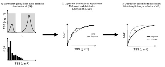
In this study, stormwater quality models are calibrated using a distribution-based approach depicted in Figure 1. Instead of replicating single-event characteristics or pollutographs, the approach aims to minimize the difference between observed and simulated TSS event load distribution. Since observed TSS event load distributions can be well approximated with theoretical distribution functions [22], the calibration uses a site-specific parameterized lognormal distribution as reference (cf. Section 2.3). The approach focuses on probabilistic event load distribution and places less emphasis on intra-event dynamics. Model results therefore need to be analyzed by means of mass-volume curves (MV curves) [23].
2.2. Experimental Sites and Measurement Data
Stormwater runoff and quality processes of a flat roof (FR, 50 m2) and a parking lot (PL, 2350 m2) are considered. At both sites, a long-term online monitoring campaign has been conducted and continuous runoff and quality data at the outlet of the catchment was collected [24]. Stormwater quality data are available from March 2013–November 2015 (stormwater quality observation period). Rainfall measurement is still operated.
Based on site-specific correlation functions for the relationship of TSS and turbidity, continuous TSS time series were estimated from online turbidity measurements. Measurement data were subjected to statistical analysis which is presented and discussed in Leutnant et al. [24]. The authors successfully measured 65 rainfall-runoff events at site FR and 46 events at site PL. The average of all event mean concentrations (µEMC) is 33 mg L−1 at site FR and 60 mg L−1 at site PL. Summing up the estimated TSS loads of all observed events yields 11.3 g m−2 at site FR and 10.6 g m−2 at site PL. Table 1 shows a summary of site and stormwater quality measurement data. Table 2 summarizes rainfall characteristics within and after the stormwater quality observation period. Detailed descriptive event statistics of rainfall, runoff, and TSS loads are given in Leutnant et al. [24].
2.3. Theoretical Distribution Function for Site-Specific TSS Event Loads
Leutnant et al. [22] use TSS event load data from Leutnant et al. [24] and describe site-specific empirical TSS event load distributions by means of theoretical distribution functions. The authors demonstrated that the two-parameter lognormal distribution approximates the empirical TSS event load distribution well and can therefore be used to probabilistically describe TSS event loads. In their study, parameters of the lognormal distribution are optimized with respect to a likelihood function and the goodness-of-fit is evaluated by means of Kolmogorov–Smirnov and Anderson–Darling test statistics. Table 3 shows the general lognormal distribution formula and optimized parameter for μ (meanlog) and σ (sdlog) for sites FR and PL taken from Leutnant et al. [22].
2.4. Stormwater Quality Modelling
In this study, pollutant processes for buildup and wash-off are modelled with the widely used exponential equations implemented in the stormwater management model SWMM5 [25]. Buildup B(t) is mathematically described as a function of antecedent dry weather days t (Equation (1)). Pollutant wash-off W(t) is expressed as a function of the current runoff rate q(t) and available masses on the surface B(t) (Equation (2)). Both functions offer two individual parameters to be calibrated. Additionally, the initial buildup B0 at the beginning of the simulation (t = 0) needs to be estimated.
Table 4 shows the parameter used for calibration. Corresponding parameter ranges were extracted from the literature [5,26] and harmonized with the authors’ experience.
with buildup coefficient k (g m−2), buildup exponent α (d−1), t denotes the number of preceding dry weather days.
with wash-off coefficient C1(-), wash-off exponent C2(-), runoff rate q (mm h−1), available pollutant masses on the surface B (g m−2), and time index t.
2.5. Parameter Estimation and Goodness-of-Fit Assessment
For both sites, model parameters affecting runoff generation and hydrograph characteristics are initially calibrated by means of the multi-objective algorithm NSGA-2 [27]. The algorithm allows to optimize multiple objectives simultaneously and identifies Pareto-optimal solutions from which a compromise can be drawn. Here, a single objective is defined as an event-specific Nash–Sutcliffe Efficiency (NSE) [28]. Eight representative rainfall-runoff events were taken into account which consequently yields eight objectives to be optimized. Rainfall events have a minimum depth of 2 mm and a minimum intensity in 60 min of 2.5 mm h−1. The compromise solution follows the L2-metric [29] which calculates the Euclidean distance of all pareto-optimal solutions to an ideal solution. The solution with the smallest Euclidean distance is considered as a compromise. Model parameters (i) surface roughness; (ii) depression storage and (iii) characteristic width of the overland flow are considered for calibration. The calibration yielded an average event-specific NSE of 0.73 for site FR and 0.72 for site PL (the results of water quantity calibration are not further discussed in this paper).
Once optimized parameters of runoff calibration are estimated, model parameters for pollutant buildup and wash-off (cf. Table 4) are optimized. The calibration aim is to fit the simulated TSS event load distribution to the parameterized lognormal distribution. For this purpose, the Kolmogorov–Smirnov (KS) statistic Dn which numerically describes the equality of two distributions and tests whether a sample follows a specific distribution [30] is used as the objective function. This means that the smaller the KS statistic Dn becomes, the higher the goodness-of-fit of the calibration. The KS statistic ranges from 0 ≤ Dn ≤ 1. As this calibration only considers a single objective, a single objective optimization algorithm is used. A differential evolution algorithm [31] implemented by Ardia et al. [32] is applied. The following computation steps are performed:
- Simulation with a new set of parameters generated by the optimization algorithm.
- Determine and split events from simulation time series which satisfy selection criteria (Table 5). An event starts when runoff starts and ends if the maximum runoff within a predefined window is 0.
- Computation of runoff volume and TSS load per event.
- Selection of events which exceeds a minimum runoff volume (Table 5). This step is introduced because the small size of the catchments leads to a significant number of events with numerically low runoff volume which would result in weights that are disproportionate to these events.
- Computation of the cumulative TSS event load distribution function for the events remaining.
- Computation of Kolmogorov–Smirnov Distance Dn according to Equation (3):with FSWMM being the simulated cumulative TSS event load distribution function and Flognormal the site-specific parameterized lognormal distribution function.
- Repeat steps 1–7 to minimize Dn until convergence.
The goodness-of-fit of the calibrated stormwater quality model is numerically assessed and visually evaluated through a direct comparison of the simulated distribution function and the parameterized lognormal distribution function for TSS event loads. Residuals of the simulated event loads and observed event loads are computed. Simulated intra-event dynamics are analyzed by means of mass-volume curves (MV curves).
2.6. Concept of Model Validation
The calibration uses measurement data from the site-specific stormwater quality observation period. Estimated parameters are expected to be valid beyond this period. The model validation therefore uses all available rainfall data from the five-year period (March 2013–April 2018, cf. Table 1). Equality of simulated TSS event load distributions from the five-year period and the observation period are evaluated using Kolmogorov–Smirnov’s distance KS DN.
2.7. Model Parameter Uncertainty Analysis
The differential evolution algorithm applied belongs to the class of genetic algorithms which minimize an objective function by evolving a population of candidate solutions through successive generations [32]. In this study, the configuration of evolution strategy and mutating operators (crossover probability and differential weighting factor) follows the developer’s recommendation. However, the maximum number of iterations is set to 400 and the number of population members (i.e., parameter sets per iteration) is set to 100, which results in 40,000 simulation runs per model in total. For estimating model parameter uncertainties, simulation results are divided into behavioral and non-behavioral groups. Parameter sets that yield the best 20% solutions are attributed as behavioral and subjected to descriptive statistical analysis (mean, standard deviation, and coefficient of variation).
2.8. Estimation of Annual TSS Event Loads
The calibrated stormwater quality models are further used to estimate annual TSS event loads and event mean concentrations originated from the study sites. Annual TSS event loads are estimated by considering all event loads from a moving window of 12 consecutive months to account for natural rainfall variability. Using the extended rainfall series, the simulation period comprises ca. five years, with 62 months which yields 50 (62–12) moving years.
3. Results and Discussion
Calibration results for both sites are shown in Table 6. Statistics for both model parameters and the Kolmogorov–Smirnov-based objective function are given. The best fit parameter sets yielded to an objective function of roughly 0.05 for both models.
According to the low Kolmogorov–Smirnov statistic Dn of approx. 0.05 for both sites, the best-fit parameter sets obtained by the distribution-based calibration approach lead to well-approximated parameterized lognormal distributions. From a statistical perspective which also takes the number of samples into account, it can be legitimately assumed that both distributions (lognormal and simulated TSS event loads) follow the same distribution. Both KS statistics are below the critical values at the 90% significance level (0.082 for site FR and 0.118 at site PL).
Distributions of simulated and observed event mean concentrations (EMC) are compared in Table 7. A notably high agreement of mean EMC is obtained for both sites (FR: 33 mg L−1, PL: 62 mg L−1). It can also be observed that EMC percentiles of simulation for site FR are slightly higher than the observed percentiles until the 0.75 percentile. Site PL shows the opposite behavior: EMC percentiles of simulation are slightly lower than observed percentiles until the 0.5 percentile. However, in both cases, the maximum observed EMC percentiles are strongly underestimated which suggests an inappropriate accumulation process model to account for random influences (e.g., traffic-induced pollutant emissions [33]).
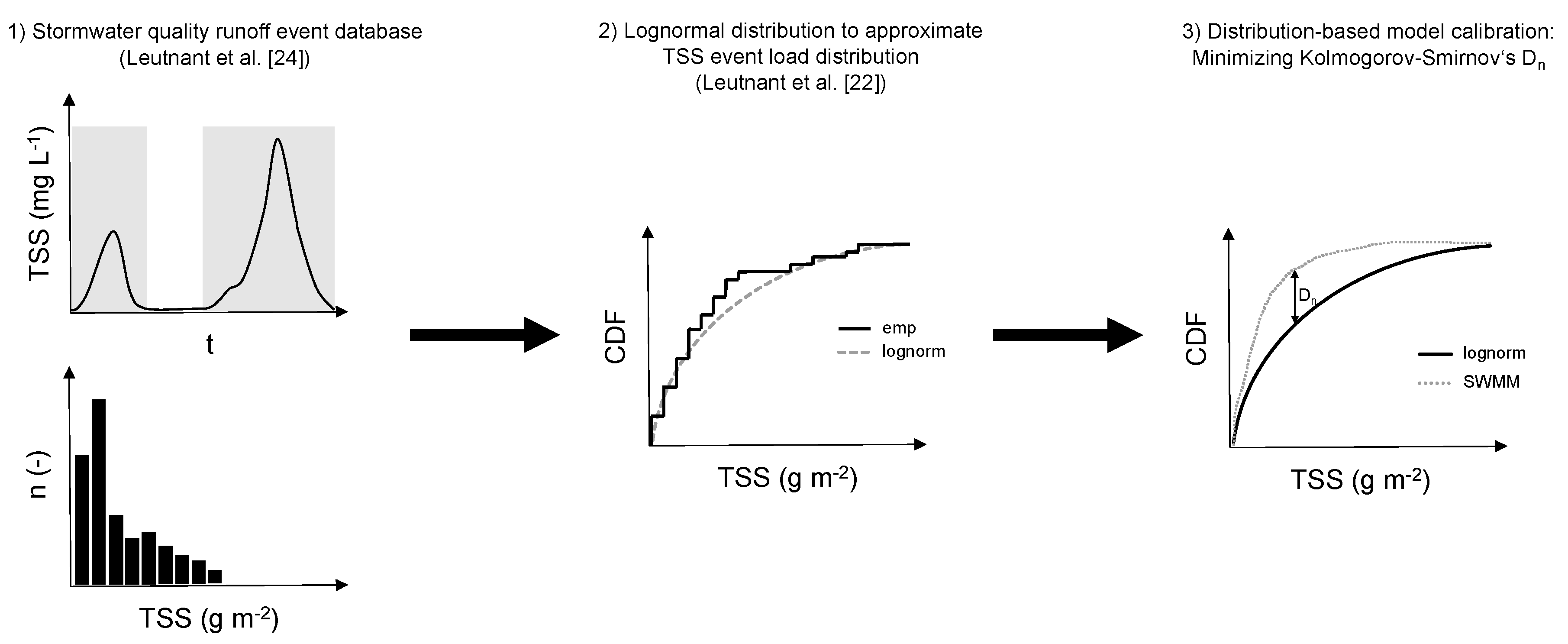
The fact that events with high TSS event mean concentrations are underestimated affects the goodness-of-fit concerning the total TSS event load of the events observed (Table 8). This is especially evident at site PL, where the total TSS event load is underestimated by roughly 28%. Events with more than 0.5 g m−2 are poorly represented (cf. Figure 2).
At site FR, the relative deviation is only about 5%. This signals that the error is compensated by events whose simulated TSS event load is higher than that which is observed (intersection at approx. 0.1 g m−2, cf. Figure 2).
Cumulative distribution functions of simulated TSS event loads are depicted for both models in Figure 2. Simulation results are opposed to the parameterized lognormal distribution function used for calibration and the original empirical distribution function from observation. Additionally, absolute residuals between observed and simulated TSS event loads are presented on the right-hand side of the figure (FR: subplot (b), PL: subplot (d)). At site FR, the mean of TSS event load residuals is −0.0087 g m−2 (sd: 0.19; min: −0.41; max: 0.94). At site PL, the mean of the TSS event load residuals is 0.065 g m−2 (sd: 0.19; min: −0.27; max: 0.74).
At site FR, the calibrated model replicates the distribution function until the 0.8 percentile with a high goodness-of-fit. Events exceeding this value are generally underestimated by the model and lead to lower simulated event loads than suggested by the lognormal distribution. Since the KS statistic represents the maximum distance between two cumulative distribution functions, the maximum 5% of the events with more than the 0.8 percentile of event loads are underestimated.
The results for site PL show a similar effect. Here, the model shows a good fitting of the distribution function until the 0.9-percentile, which accordingly implies that the maximum 5% of the events with more than the 0.9-percentile of event loads are underestimated.
Both calibrated models tend to underestimate events with high TSS loads which indicates that the calibration approach and the objective function applied is heavily influenced by events with low TSS event load which, as a matter of fact, is the case for the majority of events for both sites. Applying an alternative goodness-of-fit measure as an objective function, which also emphasizes the upper tailing of a distribution function could lead to superior model performance. This, however, remains unclear as the applied pollutant model itself also has limitations in replicating natural pollutant processes [5,12,34].
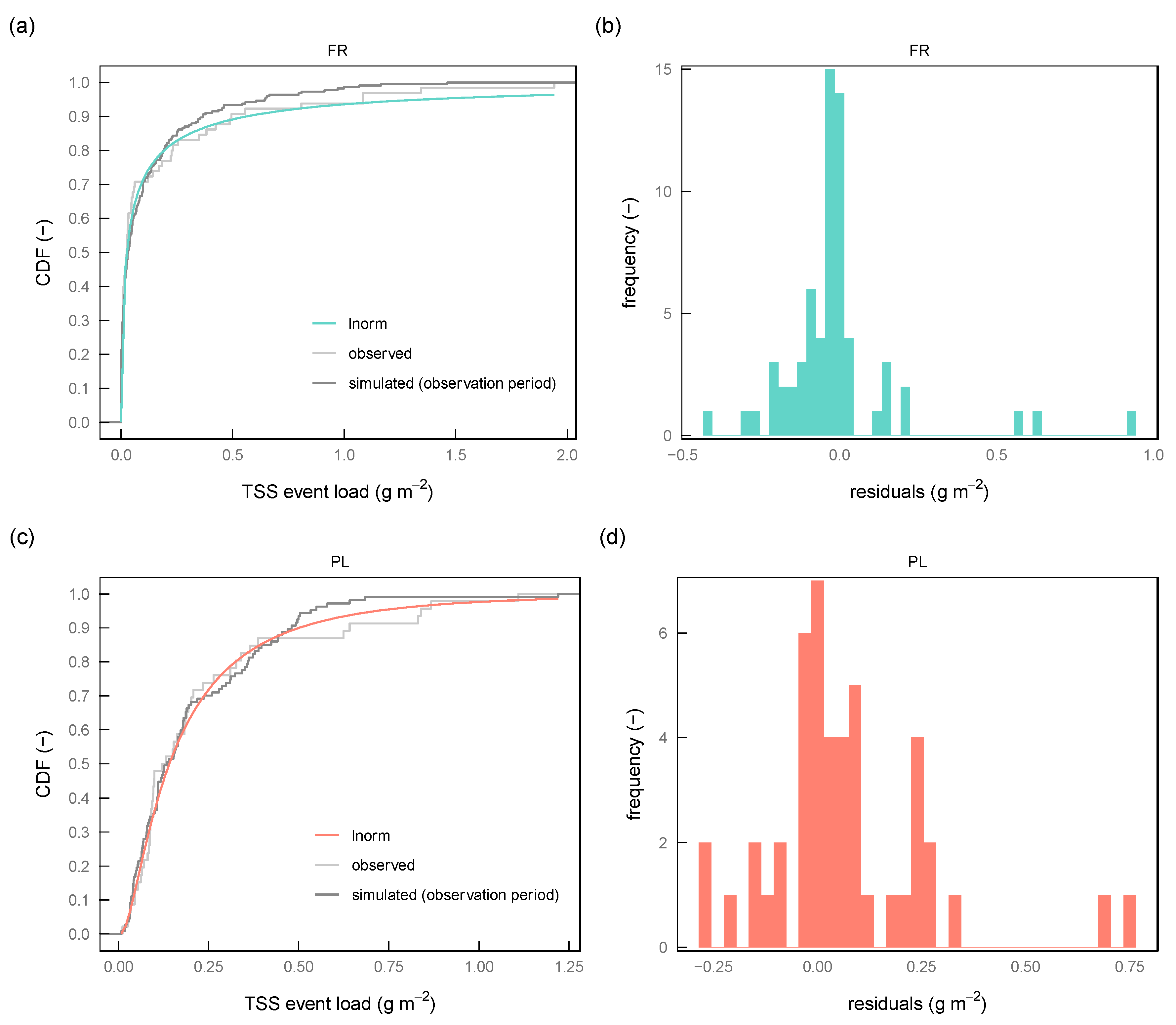
Observed and simulated MV curves are shown in Figure 3. Simulated MV curves are calculated for both the stormwater quality observation period and the five-year period using all available rainfall data.
Mass-volume curves for site FR reveal that simulated intra-event processes do not reflect the observed dynamics in general. In particular, the prevailing first-flush characteristic is not appropriately replicated. Instead, simulated wash-off tends to occur proportionally to runoff.
In contrast, statistics of simulated intra-event processes at site PL correspond well to the data observed. It can be seen that the calibrated model also tends to generate wash proportional to runoff. The high agreement of observed and simulated MV curves at site PL is obtained since the observed MV curves already show a more runoff-proportional wash-off behavior. Although the general characteristic at site PL is satisfactorily represented, the results from both sites indicate that the observed intra-event dynamic can hardly be deterministically described by the model for a continuous simulation period. As pointed out in previous studies [5,12], pollutant buildup and wash-off are highly affected by stochastic inputs, which consequently limits the goodness-of-fit of replicating intra-event dynamics.
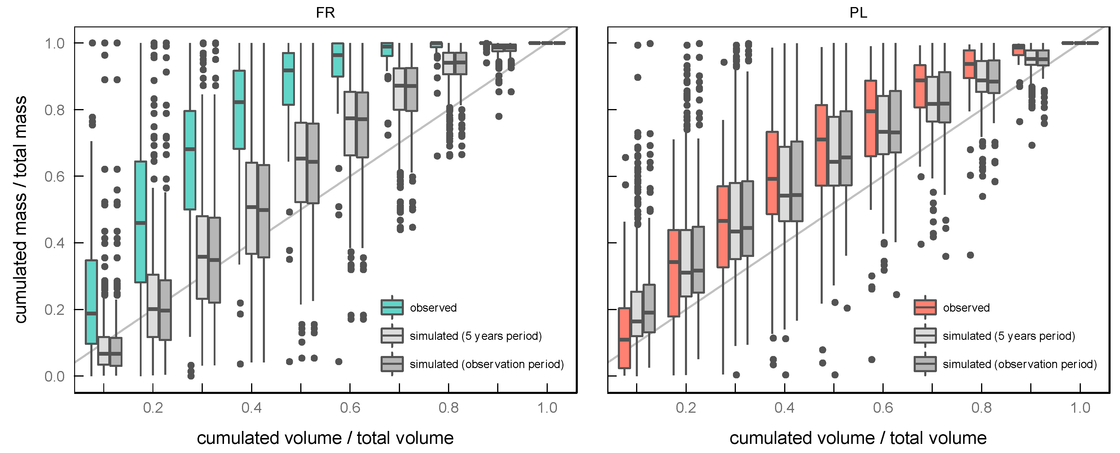
Simulated distribution functions from the observation period (used for calibration) are compared to the results using the five-year period (validation) in Figure 4. Corresponding goodness-of-fit is given in Table 9.
At site FR, the KS statistic between both distributions is 0.035, implying that the observation period is highly representative. The KS statistic of 0.062 from validation only slightly differs from calibration (KS: 0.053), which indicates a successful model validation.
In contrast, the distribution function from validation at site PL constantly underestimates the assumed lognormal distribution. This is also expressed by a higher KS statistic of 0.073. The distance between calibration and the validation period is slightly higher (KS: 0.083), indicating a less successful model validation. However, it is noticeable that the simulated TSS event distribution of the observation period falls below the lognormal distribution between 0.25 g m−2 and 0.4 g m−2 and exceeds the lognormal distribution for event loads higher than 0.5 g m−2. This indicates that the observation period is less representative as the number of events is significantly lower.
The validated models were finally used to estimate annual TSS loads (Table 10) which is of special interest for practical purposes. In the present study, the estimated mean annual TSS load for site FR is 9.9 g m−2 a−1 which according to Dierschke [35] represents a roof with “low to normal” load contribution. The annual TSS load for site PL was estimated at 13.7 g m−2 a−1, which is significantly lower than reported from measurements by Burton and Pitt [36] (~40 g m−2 a−1). As already stated, the model disregards traffic-related stochastic inputs, which could explain the low annual TSS loads estimated. Consequently, the result must be carefully interpreted. This highlights the need to especially account for load-intensive events either through an alternative objective function or modification of the model concept which, e.g., occasionally allows the incorporation of pollutants from additional sources.
Generally, the distribution-based calibration approach allows to calibrate stormwater quality models even if data is incomplete but tends to underestimate events with high TSS loads. However, compared to the conventional calibration, the approach has two clear advantages. First, the occurrence of events and its corresponding pollutant contribution is probabilistically considered, which implies that stochasticity is taken into account. Second, measurement data of stormwater quality processes are rarely completely available for continuous periods which consequently complicates the application of a conventional calibration approach and could result in misleading model outputs. Theoretical distribution functions are continuously defined.
4. Conclusions
An innovative calibration approach for stormwater quality models with respect to TSS event load distribution is introduced. The approach was applied on two experimental sites, (i) flat roof and (ii) parking lot, for which parameterized lognormal distribution functions were available. From this study, the following can be concluded:
- Both models have been successfully calibrated, as indicated by the low Kolmogorov–Smirnov distance measure. TSS event load distribution functions from calibration period were compared to distribution functions obtained from simulation with extended rainfall data.
- Maximum deviation between lognormal and simulated TSS event load distribution is 5%.
- A high agreement of the observed and simulated mean of event mean concentrations (µEMC) was achieved for both sites (FR: 33.2 vs. 33.4 mg L−1, PL: 60.3 vs. 62.9 mg L−1).
- Using a theoretical distribution for calibration provides continuous probabilities and allows to calibrate stormwater quality models even if data is incomplete.
- The approach is generally applicable and especially powerful if distribution functions become generalizable on a catchment-scale.
- The objective function used for calibration employs the Kolmogorov–Smirnov statistic. Despite its simplicity, it has been shown that events with high TSS event loads tend to be underestimated. A more behavioral distance measure which also accounts for events with high loads remains open for future research.
- Based on the calibrated models, annual TSS event loads were estimated. A load of 9.9 g m−2 a−1 was obtained for the flat roof site, and 13.7 g m−2 a−1 was obtained for the parking lot site.
The calibration approach still needs to be tested on larger catchments which consist of multiple subcatchments with different land uses. This requires catchment-specific theoretical distribution functions to be available. Additionally, it could be of interest to determine whether model parameters are correlated to parameters of the theoretical distribution function or catchment characteristics.
Author Contributions
D.L., D.M. and M.U. conceived and designed the numerical experiments; D.L. performed the numerical computations and evaluated the results; D.L. wrote the paper; and thanks are given to D.M. and M.U. for professional discussions.
Funding
The research is part of the project “Modelle für Stofftransport und -behandlung in der Siedlungshydrologie” (STBMOD) at the Institute for Infrastructure, Water, Resources, and Environment, Muenster University of Applied Sciences. The project was funded by the German Federal Ministry of Education and Research (BMBF, FKZ 03FH033PX2).
Acknowledgments
The authors would like to thank the four anonymous reviewers for their valuable comments.
Conflicts of Interest
The authors declare no conflict of interest.
References
- Dotto, C.B.S.; Kleidorfer, M.; Deletic, A.; Rauch, W.; McCarthy, D.T.; Fletcher, T.D. Performance and sensitivity analysis of stormwater models using a Bayesian approach and long-term high resolution data. Environ. Model. Softw. 2011, 26, 1225–1239. [Google Scholar] [CrossRef]
- Dotto, C.B.S.; Deletic, A.; Fletcher, T.D. Analysis of parameter uncertainty of a flow and quality stormwater model. Water Sci. Technol. 2009, 60, 717–725. [Google Scholar] [CrossRef] [PubMed]
- Sartor, J.D.; Boyd, G.B. Water Pollution Aspects of Street Surface Contaminants; US Environmental Protection Agency: Washington, DC, USA, 1972.
- Muschalla, D.; Schneider, S.; Gamerith, V.; Gruber, G.; Schroter, K. Sewer modelling based on highly distributed calibration data sets and multi-objective auto-calibration schemes. Water Sci. Technol. 2008, 57, 1547–1554. [Google Scholar] [CrossRef] [PubMed]
- Sage, J.; Bonhomme, C.; Al Ali, S.; Gromaire, M.-C. Performance assessment of a commonly used “accumulation and wash-off” model from long-term continuous road runoff turbidity measurements. Water Res. 2015, 78, 47–59. [Google Scholar] [CrossRef] [PubMed] [Green Version]
- Bonhomme, C.; Petrucci, G. Should we trust build-up/wash-off water quality models at the scale of urban catchments? Water Res. 2017, 108, 422–431. [Google Scholar] [CrossRef] [PubMed]
- Egodawatta, P.; Thomas, E.; Goonetilleke, A. Mathematical interpretation of pollutant wash-off from urban road surfaces using simulated rainfall. Water Res. 2007, 41, 3025–3031. [Google Scholar] [CrossRef] [PubMed] [Green Version]
- Muthusamy, M.; Tait, S.; Schellart, A.; Beg, M.N.A.; Carvalho, R.F.; de Lima, J.L.M.P. Improving understanding of the underlying physical process of sediment wash-off from urban road surfaces. J. Hydrol. 2018, 557, 426–433. [Google Scholar] [CrossRef] [Green Version]
- Zhao, J.; Chen, Y.; Hu, B.; Yang, W. Mathematical Model for Sediment Wash-Off from Urban Impervious Surfaces. J. Environ. Eng. 2015, 142, 04015091. [Google Scholar] [CrossRef]
- Alias, N.; Liu, A.; Goonetilleke, A.; Egodawatta, P. Time as the critical factor in the investigation of the relationship between pollutant wash-off and rainfall characteristics. Ecol. Eng. 2014, 64, 301–305. [Google Scholar] [CrossRef] [Green Version]
- Zhao, H.; Jiang, Q.; Xie, W.; Li, X.; Yin, C. Role of urban surface roughness in road-deposited sediment build-up and wash-off. J. Hydrol. 2018, 560, 75–85. [Google Scholar] [CrossRef]
- Shaw, S.B.; Stedinger, J.R.; Walter, M.T. Evaluating Urban Pollutant Buildup/Wash-Off Models Using a Madison, Wisconsin Catchment. J. Environ. Eng. 2010, 136, 194–203. [Google Scholar] [CrossRef]
- Harremoës, P. Stochastic models for estimation of extreme pollution from urban runoff. Water Res. 1988, 22, 1017–1026. [Google Scholar] [CrossRef]
- Scholz, K. Stochastische Simulation Urbanhydrologischer Prozesse (“Stochastic Simulation of Urban Hydrological Processes”). Ph.D. Thesis, University of Hannover, Hannover, Germany, 1995. (In German). [Google Scholar]
- Osman Akan, A. Derived Frequency Distribution for Storm Runoff Pollution. J. Environ. Eng. 1988, 114, 1344–1351. [Google Scholar] [CrossRef]
- Rossi, L.; Krejci, V.; Rauch, W.; Kreikenbaum, S.; Fankhauser, R.; Gujer, W. Stochastic modeling of total suspended solids (TSS) in urban areas during rain events. Water Res. 2005, 39, 4188–4196. [Google Scholar] [CrossRef] [PubMed]
- Chen, J.; Adams, B.J. A derived probability distribution approach to stormwater quality modeling. Adv. Water Resour. 2007, 30, 80–100. [Google Scholar] [CrossRef]
- Sharifi, S.; Massoudieh, A.; Kayhanian, M. A Stochastic Stormwater Quality Volume-Sizing Method with First Flush Emphasis. Water Environ. Res. 2011, 83, 2025–2035. [Google Scholar] [CrossRef] [PubMed]
- Daly, E.; Bach, P.M.; Deletic, A. Stormwater pollutant runoff: A stochastic approach. Adv. Water Resour. 2014, 74, 148–155. [Google Scholar] [CrossRef]
- Qin, H.; Tan, X.; Fu, G.; Zhang, Y.; Huang, Y. Frequency analysis of urban runoff quality in an urbanizing catchment of Shenzhen, China. J. Hydrol. 2013, 496, 79–88. [Google Scholar] [CrossRef] [Green Version]
- Hannouche, A.; Chebbo, G.; Joannis, C.; Gasperi, J.; Gromaire, M.-C.; Moilleron, R.; Barraud, S.; Ruban, V. Stochastic evaluation of annual micropollutant loads and their uncertainties in separate storm sewers. Environ. Sci. Pollut. Res. 2017, 24, 28205–28219. [Google Scholar] [CrossRef] [PubMed]
- Leutnant, D.; Muschalla, D.; Uhl, M. Statistical Distribution of TSS Event Loads from Small Urban Environments. Water 2018, 10, 769. [Google Scholar] [CrossRef]
- Bertrand-Krajewski, J.L.; Chebbo, G.; Saget, A. Distribution of pollutant mass vs. volume in stormwater discharges and the first flush phenomenon. Water Res. 1998, 32, 2341–2356. [Google Scholar] [CrossRef]
- Leutnant, D.; Muschalla, D.; Uhl, M. Stormwater Pollutant Process Analysis with Long-Term Online Monitoring Data at Micro-Scale Sites. Water 2016, 8, 299. [Google Scholar] [CrossRef]
- Rossman, L.A. Storm Water Management Model—User’s Manual Version 5.0; United States Environmental Protection Agency (US EPA): Cincinnati, OH, USA, 2010; p. 285.
- Gamerith, V.; Neumann, M.B.; Muschalla, D. Applying global sensitivity analysis to the modelling of flow and water quality in sewers. Water Res. 2013, 47, 4600–4611. [Google Scholar] [CrossRef] [PubMed]
- Deb, K.; Agrawal, S.; Pratap, A.; Meyarivan, T. A Fast Elitist Non-Dominated Sorting Genetic Algorithm for Multi-Objective Optimization: NSGA-II. In Proceedings of the Parallel Problem Solving Form Nature VI Conference, Paris, France, 18–20 September 2000; Springer: New York, NY, USA, 2000; Volume 1917. [Google Scholar]
- Nash, J.E.; Sutcliffe, J.V. River flow forecasting through conceptual models part I—A discussion of principles. J. Hydrol. 1970, 10, 282–290. [Google Scholar] [CrossRef]
- Deb, K. Multi-Objective Optimization Using Evolutionary Algorithms; John Wiley & Sons, Ltd.: Chichester, UK, 2008; ISBN 978-0-470-74361-4. [Google Scholar]
- Hedderich, J.; Sachs, L. Angewandte Statistik: Methodensammlung mit R; 14., Überarb. und erg. Aufl.; Springer: Heidelberg, Germany, 2012; ISBN 978-3-642-24400-1. [Google Scholar]
- Price, K.V.; Storn, R.M.; Lampinen, J.A. Differential Evolution: A Practical Approach to Global Optimization; Natural Computing Series; Springer: Berlin, Germany; New York, NY, USA, 2005; ISBN 978-3-540-20950-8. [Google Scholar]
- Ardia, D.; Mullen, K.M.; Peterson, B.G.; Ulrich, J. DE-Optim: Differential Evolution in R. Available online: https://cran.r-project.org/package=DEoptim (accessed on 2 August 2018).
- Gunawardena, J.M.A.; Liu, A.; Egodawatta, P.; Ayoko, G.A.; Goonetilleke, A. Influence of Traffic and Land Use on Urban. Stormwater Quality—Implications for Urban Stormwater Treatment Design; SpringerBriefs in Water Science and Technology; Springer: Singapore, 2018; ISBN 978-981-10-5301-6. [Google Scholar]
- Bertrand-Krajewski, J.-L. Stormwater pollutant loads modelling: Epistemological aspects and case studies on the influence of field data sets on calibration and verification. Water Sci. Technol. 2007, 55, 1–17. [Google Scholar] [CrossRef] [PubMed]
- Dierschke, M. Methodischer Ansatz zur Quantifizierung von Feinpartikeln (PM63) in Niederschlagsabflüssen in Abhängigkeit von der Herkunftsfläche (“Methodical Approach for Quantifying of Fine Particles (PM63) in Rainfall Runoffs Depending on the Surface of Origin”). Ph.D. Thesis, University of Kaiserslautern, Kaiserslautern, Germany, 2014. (In German). [Google Scholar]
- Allen Burton, G.; Pitt, R. Stormwater Effects Handbook: A Toolbox for Watershed Managers, Scientists, and Engineers; CRC Press: Boca Raton, FL, USA, 2001; ISBN 978-0-87371-924-7. [Google Scholar]
Figure 1.
Concept of distribution-based model calibration: Observed TSS event loads are approximated by means of a lognormal distribution. During model calibration, stormwater quality model parameters are modified to minimize the distance of the simulated TSS event load distribution and the lognormal distribution. The Kolmogorov–Smirnov test statistic is used as a distance measure. (TSS: total suspended solids, CDF: cumulative distribution function, emp: empirical distribution function, lognorm: lognormal distribution, SWMM: stormwater management model).

Figure 2.
Cumulative distribution functions of lognormal, observed and simulated TSS event loads at sites flat roof (FR) (a) and parking lot (PL) (c), and the distribution of residuals between the observed and simulated event loads at sites flat roof (b) and parking lot (d).
Figure 2.
Cumulative distribution functions of lognormal, observed and simulated TSS event loads at sites flat roof (FR) (a) and parking lot (PL) (c), and the distribution of residuals between the observed and simulated event loads at sites flat roof (b) and parking lot (d).

Figure 3.
Comparison of observed and simulated mass-volume curves for sites flat roof (left) and parking lot (right).
Figure 3.
Comparison of observed and simulated mass-volume curves for sites flat roof (left) and parking lot (right).

Figure 4.
Cumulative distribution functions of lognormal and simulated TSS event loads for the observation period (calibration) and the five-year period (validation) for sites flat roof (left) and parking lot (right).
Figure 4.
Cumulative distribution functions of lognormal and simulated TSS event loads for the observation period (calibration) and the five-year period (validation) for sites flat roof (left) and parking lot (right).


Table 1.
Characteristics of experimental sites and summary of measurement data obtained.
| Parameter | Flat Roof | Parking Lot |
|---|---|---|
| area (m2) | 50 | 2350 |
| surface type (-) | Bitumen sheeting (100%) | asphalt (55%), porous pavement (40%), vegetated areas (5%) |
| slope (%) | 2 | 2.5 |
| stormwater quality observation period (-) | March 2013–November 2015 | April 2013–October 2014 |
| valid events observed (-) | 65 | 46 |
| total TSS loads of valid events (g m−2) | 11.3 | 10.6 |
| average TSS event mean concentration of valid events observed (mg L−1) | 33 | 60 |
Table 2.
Summary of rainfall characteristics within and after stormwater quality observation period.
Table 2.
Summary of rainfall characteristics within and after stormwater quality observation period.
| Period | Months | Rainfall (mm per period) | Stormwater Quality Observation Period? |
|---|---|---|---|
| March 2013–December 2013 | 10 | 475 | yes |
| January 2014–December 2014 | 12 | 897 | |
| January 2015–November 2015 | 11 | 726 | |
| December 2015 | 1 | 42 | no |
| January 2016–December 2016 | 12 | 700 | |
| January 2017–December 2017 | 12 | 734 | |
| January 2018–April 2018 | 4 | 203 |
Table 3.
Lognormal distribution function and optimized parameters to describe TSS event load distribution for site FR and PL from Leutnant et al. [22].
Table 3.
Lognormal distribution function and optimized parameters to describe TSS event load distribution for site FR and PL from Leutnant et al. [22].
| Formula | Optimized Parameter | |||
|---|---|---|---|---|
| Flat Roof | Parking Lot | |||
| μ | σ | μ | σ | |
| −3.69 | 2.429 | −1.96 | 0.987 | |
Table 4.
Quality model parameters and corresponding ranges used for calibration.
| Parameter | Description | Unit | Range |
|---|---|---|---|
| B0 | masses available at the beginning of simulation (t = 0) | g m−2 | [1; 5] |
| k | maximum possible buildup | g m−2 | [0.0001; 2] |
| α | rate constant of buildup per day | d−1 | [0.0001; 0.2] |
| C1 | wash-off coefficient | - | [0.0001; 1] |
| C2 | wash-off exponent | - | [0.0001; 3] |
Table 5.
Summary of the simulation period and rainfall-runoff event selection criteria.
| Flat Roof | Parking Lot | |
|---|---|---|
| Simulation duration (observation period) | March 2013–November 2015 | April 2013–October 2014 |
| Simulation duration (a) | 2.7 | 1.6 |
| Days with rainfall ≥ 2 mm d−1 | 250 | 137 |
| Event selection criteria | ||
| Event window (min) | 480 | |
| Min. Runoff volume (l) | 19 (~0.4 percentile) | 465 (~0.2 percentile) |
| Events selected (-) | 224 | 107 |
Table 6.
Calibrated model parameters and corresponding uncertainty statistics (FR: flat roof, PL: parking lot, sd: standard deviation, CoV: coefficient of variation, KS Dn: Kolmogorov–Smirnov distance).
Table 6.
Calibrated model parameters and corresponding uncertainty statistics (FR: flat roof, PL: parking lot, sd: standard deviation, CoV: coefficient of variation, KS Dn: Kolmogorov–Smirnov distance).
| Objective Function | Parameter | ||||||
|---|---|---|---|---|---|---|---|
| Site | Statistic | KS Dn | B0 | k | α | C1 | C2 |
| - | g m−2 | g m−2 | d−1 | - | - | ||
| FR | best fit | 0.053 | 2.713 | 1.899 | 0.022 | 0.017 | 2.040 |
| mean | 0.056 | 3.437 | 1.706 | 0.024 | 0.021 | 2.070 | |
| sd | 0.003 | 0.608 | 0.201 | 0.005 | 0.006 | 0.054 | |
| CoV | 0.053 | 0.177 | 0.118 | 0.212 | 0.277 | 0.026 | |
| PL | best fit | 0.049 | 4.545 | 0.891 | 0.194 | 0.472 | 1.120 |
| mean | 0.050 | 4.726 | 0.882 | 0.204 | 0.470 | 1.103 | |
| sd | 0.002 | 0.257 | 0.053 | 0.021 | 0.043 | 0.070 | |
| CoV | 0.032 | 0.054 | 0.061 | 0.105 | 0.091 | 0.063 | |
Table 7.
Observed (obs) and simulated (sim) TSS event mean concentrations (observed values are taken from [24]).
Table 7.
Observed (obs) and simulated (sim) TSS event mean concentrations (observed values are taken from [24]).
| Site | Source | n | TSS Event Mean Concentration (mg L−1) | ||||||||
|---|---|---|---|---|---|---|---|---|---|---|---|
| Min | 0.1-Perc. | 0.25-Perc. | Median | 0.75-Perc | 0.9-Perc. | Max | Mean | Sd | |||
| FR | obs | 65 | <0.1 | 1.2 | 2.8 | 9.0 | 35.1 | 94.0 | 249.9 | 33.2 | 54.6 |
| sim | 65 | 1.2 | 5.8 | 9.6 | 20.6 | 35.5 | 82.6 | 178.2 | 33.4 | 36.5 | |
| PL | obs | 46 | 4.7 | 13.2 | 24.4 | 49.4 | 80.1 | 112.4 | 253.7 | 60.3 | 49.3 |
| sim | 46 | 0.2 | 4.6 | 13.9 | 45.4 | 98.8 | 156.6 | 161.6 | 62.9 | 54.7 | |
Table 8.
Observed and simulated total TSS event loads (observed values are taken from [24]).
Table 8.
Observed and simulated total TSS event loads (observed values are taken from [24]).
| Site | Events | Total TSS Event Loads (g m−2) | ||
|---|---|---|---|---|
| Observed | Simulated | Relative Deviation | ||
| FR | 65 | 11.3 | 11.9 | +5% |
| PL | 46 | 10.6 | 7.57 | −28% |
Table 9.
Goodness-of-fit matrix for the observation period (calibration) and five-year period (validation) (FR: flat roof, PL: parking lot, KS Dn: Kolmogorov–Smirnov distance).
Table 9.
Goodness-of-fit matrix for the observation period (calibration) and five-year period (validation) (FR: flat roof, PL: parking lot, KS Dn: Kolmogorov–Smirnov distance).
| Site | KS Dn | ||
|---|---|---|---|
| Lnorm | Observation Period | ||
| FR | lnorm | - | |
| observation period | 0.053 | - | |
| Five-year period | 0.062 | 0.035 | |
| PL | lnorm | - | |
| observation period | 0.049 | - | |
| Five-year period | 0.073 | 0.083 | |
Table 10.
Simulated annual TSS loads (FR: flat roof, PL: parking lot).
| Site | n (Moving Years within 5 Years Period) | Annual TSS Loads (g m−2 a−1) | |
|---|---|---|---|
| Mean | sd | ||
| FR | 50 | 9.9 | 0.75 |
| PL | 50 | 13.7 | 1.17 |
© 2018 by the authors. Licensee MDPI, Basel, Switzerland. This article is an open access article distributed under the terms and conditions of the Creative Commons Attribution (CC BY) license (http://creativecommons.org/licenses/by/4.0/).
Share and Cite
MDPI and ACS Style
Leutnant, D.; Muschalla, D.; Uhl, M. Distribution-Based Calibration of a Stormwater Quality Model. Water 2018, 10, 1027. https://doi.org/10.3390/w10081027
AMA Style
Leutnant D, Muschalla D, Uhl M. Distribution-Based Calibration of a Stormwater Quality Model. Water. 2018; 10(8):1027. https://doi.org/10.3390/w10081027
Chicago/Turabian StyleLeutnant, Dominik, Dirk Muschalla, and Mathias Uhl. 2018. "Distribution-Based Calibration of a Stormwater Quality Model" Water 10, no. 8: 1027. https://doi.org/10.3390/w10081027
Note that from the first issue of 2016, this journal uses article numbers instead of page numbers. See further details here.