An Optimal Model for Water Resources Risk Hedging Based on Water Option Trading

1
College of Hydrology and Water Resources, Hohai University, No.1 Xikang Road, Nanjing 210098, China
2
National Engineering Research Center of Water Resources Efficient Utilization and Engineering Safety, Hohai University, No.1 Xikang Road, Nanjing 210098, China
3
School of Earth Sciences and Engineering, Hohai University, No.1 Xikang Road, Nanjing 210098, China
*
Author to whom correspondence should be addressed.
Water 2018, 10(8), 1026; https://doi.org/10.3390/w10081026
Submission received: 18 June 2018
/
Revised: 26 July 2018
/
Accepted: 31 July 2018
/
Published: 3 August 2018
(This article belongs to the Section Water Resources Management, Policy and Governance)
Abstract
:The uncertainty of forecasted runoffs brings risks of water shortages to water users in the intake area of long-distance water transfer projects, and the uncertainty of spot market prices may cause them to buy water at high prices. In order to hedge these risks, this paper proposes a risk hedging model for decision-making in water option trading from the viewpoint of water users. With the objective of maximizing the expected revenue of water users, the proposed model was solved by an analytical method and an optimal water option strategy was obtained for the users. The proposed model is applied to an intake area of an inter-basin water transfer project in China. The results show that the proposed water option trading model can provide water users with an optimal option strategy. The optimal options trading strategy can effectively reduce the risk caused by the uncertainties of forecasted runoffs and water prices. We also explored the influence of the uncertainty degree of the forecasted runoffs and water price on the option trading strategy. The results show that the expected revenue of water users increases as the variances of the errors of forecasted runoffs and water prices increase.
1. Introduction
To alleviate the regional water scarcity caused by climate change [1] and the uneven spatial and temporal distribution of water resources, many countries and regions have built long-distance water transfer projects. In the intake area of long-distance water transfer projects, the water supply sources of water users include local water and transferred water [2]. In order to purchase the transferred water at a lower price, water users usually sign a contract with the water supply company in advance. The optimal water purchase strategy for water users is to use the local water first, and then water shortages will be overcome by a contract of transferred water [3]. However, this simple decision process becomes complex due to the uncertainty of local water runoffs [4,5] and the fluctuation of spot market prices. These uncertainties bring risks into the decision-making for the water users. For example, the water users may be at risk of water scarcity and of high prices to buy water from the spot market if they buy less transferred water through the contracts than the demanded water. The water users will also be at risk of extra economic cost if they purchase too much transferred water through the contracts. To address the problem of water scarcity and economic loss, there is a need for more effective and flexible institutional arrangements and allocation mechanisms [6,7,8]. Water trade can help water users meet the water demand and reduce the economic loss caused by water scarcity [9]. Water trade tools, such as water banks [10,11], spot market transactions [12], virtual water [13,14] and option contracts [15,16], have been introduced by many researchers to increase water supply flexibility and reliability. Among these instruments, an option contract is the most efficient for the city water supply system. The option contract has attracted more and more interest within several water markets [15,17,18,19]. Option contracts allow the holders to delay water purchase decisions until more information is available [20] and offer protection against spot price volatility [21]. By granting users the right to buy an additional amount of water during drought periods, water option contracts are potential cost-minimizing strategies for hedging water supply risks [19]. Thus, we can use water options to hedge the risks of the contracts of transferred water. The hedging strategy for water users is to buy water options while signing a contract for transferred water. If the actual runoffs are less than the expected runoffs, the users can use the profit from the water option to make up for the loss caused by the shortage of transferred water. If the actual runoffs are more than the expected runoffs, then the users do not exercise the option and lose the premiums, but they can get compensation from the return of transferred water.
Currently, water market and option contracts are becoming more and more popular in the research field of water resources, and the water options market has wide application prospects. Research on water options has been carried out by many scholars. For instance, Holburt et al. [22] introduced the concept of options into water resources and proposed the concept of a water option contract (WSOC). Michelsen et al. [23] compared the cost of an option contract with the cost of water supply alternatives, and then proposed an economic benefit evaluation model for water supply operation. In 1994, the United States government first applied water option trading to guarantee city water supplies. The government bought water option contracts from the electric power company and paid premiums to take an option on the execution of water rights [24]. On the basis of the Black–Scholes option pricing theory, Villinski [25] constructed a multi-usage water option pricing model through numerical integration. Garrido et al. [26] developed a dynamic, stochastic, and discrete time model to characterize the contract from the viewpoint of the sellers. The model was applied to an urban water supply system in Seville to simulate city water option trading. Ranjan et al. [27] proposed a stylized mathematical simulation model which can be used to evaluate the influence of some key variables on the participation of farmers in spot and options markets. The results show that appropriate option contracts can help farmers reduce the purchase cost of water. A stochastic recursive mathematical programming model is applied to simulate the water procurement decisions of an irrigation district’s board operating in the context of water supply uncertainty in south-eastern Spain. The results suggest that the contract premium and quantity have large impacts on the decision variables [19].
However, as we can see from the above literature, research has mainly concentrated on the urban and agricultural water supply from the perspective of water management departments. The research on the combination of the spot market, contract market and options market has been limited. Therefore, based on the comparison of the expected cost of the option trading and the expected cost of the spot trading, this paper establishes a water option trading model to hedge water supply risks with the objective of maximizing the expected revenue of water users from their own perspective. The proposed model is a combined trading model of the option market, the contract market and the spot market. It is capable of exploiting the hedging of the option market, the stability of the contract market and the flexibility of the spot market. The rest of the paper is organized as follows: in Section 2, the methodology of water option trading is elaborated and the water option trading model is established. In Section 3, a case study and a discussion of the results are provided to illustrate the efficiency of the model. In Section 4, a conclusion is drawn.
2. Methodology
2.1. Concept of Water Option Contracts
The water option gives the buyer the right, but not an obligation, to purchase a certain amount of water at an agreed price in a specified future period after the buyer pays a premium to the seller [21]. The buyer has the option to exercise this right, and the seller has to follow the buyer’s choice unconditionally and sells a certain amount of water at the agreed price according to the signed contract.
A water option contract generally contains the following four elements: (1) the exercise price: The price for purchasing water specified in the option contract; (2) the premium: The fee paid by the buyer to the seller in order to get the option; (3) the water volume: The maximum amount of water that the buyer has the right to buy in the future period; and (4) the maturity date: A time or date before which the option contract must be finished or done.
The option allows the buyer to buy additional water at the maturity date at the exercise price if the actual runoffs are less than the demanded water and the spot market price is higher than the exercise price; otherwise, the buyer waives the option and loses the premium. It follows that the execution condition of water options is stricter than that of the ordinary financial options. Therefore, it is of great significance for the users to research the optimal water options trading strategies.
2.2. Two-Stage Water Option Trading Decision Model
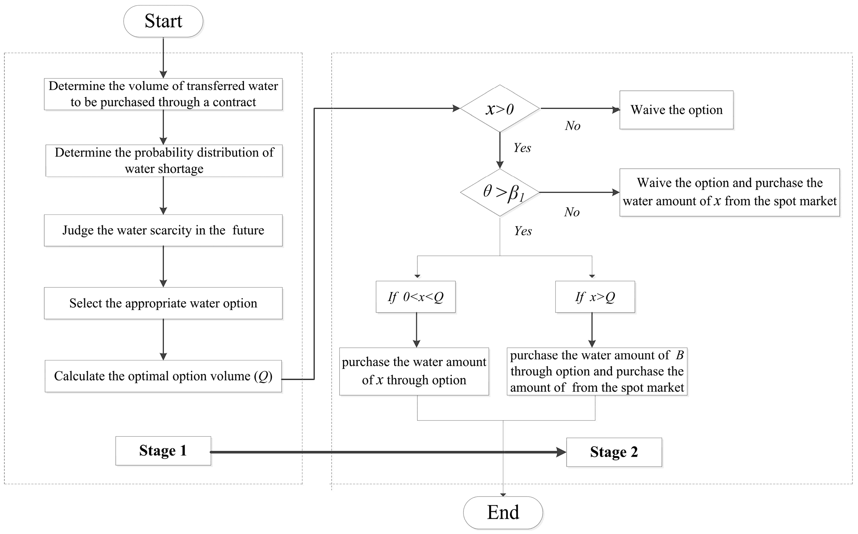
The decision-making process of water options trading is divided into two stages, as shown in Figure 1:
In the first stage, the water users should determine the volume of transferred water to be purchased through a contract based on the relation between demanded water and forecasted runoffs and get the probability distribution of water shortage. Then, the water users shall judge whether there is a water scarcity risk. If there is a water shortage risk, the users choose to buy an option contract defined as from the options market, where is the exercise price, and where is the premium. The deposit is , which is calculated according to the quantity of water () pre-purchased through the option contract and the exercise price.
In the second stage, in order to meet the water demand, water users will determine whether to execute the option at the maturity date and the water amount to buy from the spot market according to the local actual runoffs and the spot market price. Specifically, it is supposed that the spot market price at the maturity date is , and the actual water shortage for the water user is . The option is exercised if the water user is short of water and the exercise price is lower than the spot market price ( and ). In the case of , the water users purchase water amount at an exercise price of . In the case of , the users purchase water amount at the exercise price of and purchase the amount of from the spot market. In the case of , the water deficit will be completely bought from the spot market.
2.3. Description of the Uncertainties
2.3.1. Uncertainty of Water Runoffs
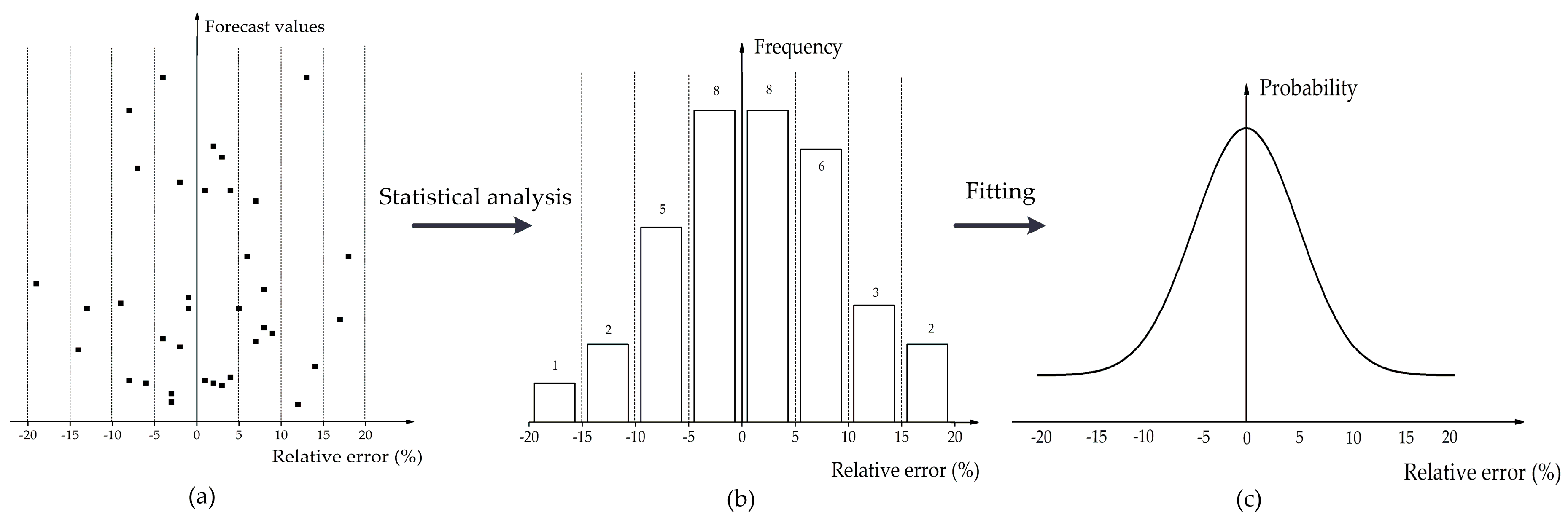
Figure 2 shows the method for deriving the relative error distribution of forecasted runoffs. As shown in Figure 2, the method consists of three components: The acquisition of forecast relative error samples, the analysis of statistical parameters, and the fitting of the distribution function of relative error.
The forecasted runoffs can be obtained by a mid-term and long-term hydrological forecast model, using the long series of historical measured runoffs data in the intake area.
However, the structure and parameter error of the hydrological prediction model lead to the error of forecasted runoffs. The relative error () of the forecasted runoffs is expressed as follows:
where refers to the measured runoffs and refers to the forecasted runoffs.
Therefore, the samples of the relative errors of the forecasted runoffs can be obtained by Equation (1).
The principle of maximum entropy (POME) is a good method to solve the problem of uncertainty. POME states that the solution of maximum entropy should be chosen from all feasible solutions. The advantages of POME are theoretical perfection and high precision. Therefore, POME is used to derive the probability density function of the relative error. According to the maximum entropy theory, the entropy of the relative error is defined as
The corresponding maximum entropy model is expressed as
where , and is the feasible set of the relative errors; is the order of the origin moment of ; is the value that makes meaningful; is the ith order origin moment of ;and is the probability density function of .
The above maximum entropy model can be solved by the Lagrange multiplier method and variational method [28]. The maximum entropy probability density function of is expressed as
where denotes Lagrange multipliers.
The forecasted runoffs in a future period are represented by . The actual runoffs are . Thus, the absolute error of is defined as , which can be derived from Equation (1), expressed as
Based on Equations (7) and (8), the probability density function () of the runoffs’ absolute error is expressed as
The total water demand of a region is affected by population size, economy of scale, planting scale and other factors. For a particular area, the changes of these elements are quite slow. Therefore, it is assumed that the total water demand () of a water user during a certain period is certain, and the water supply to the user consists of the local water, a contract of transferred water and the water purchased by options.
Based on the absolute error distribution of the forecasted runoffs, the expectation of the error is , and the expectation of the local runoffs is . Therefore, the water users can sign a contract with the supply company of water transfer project and set the amount of water purchased through the contract as .
However, the water users are still likely to be short of water after signing the contract due to the forecast errors of the local runoffs. The water deficit () is expressed as
Thus, the probability density function () of is as follows:
2.3.2. Uncertainty of Spot Market Price
The spot market price is complexly related to the supply–demand relationship, the development conditions of water resources, the quality and quantity of water resources, and owners’ equity [29]. Therefore, the spot market price is also uncertain [30]. The spot market price is affected by a combination of factors. According to the central limit theorem, when a random variable is influenced by a number of mutually independent random factors, the overall influence can be considered as being distributed in a normal state if the influence produced by each factor is not too large. Therefore, it is supposed that follows a normal distribution of . The probability density function of is as follows:
2.4. Option Trading Model Establishment and Solution
2.4.1. Optimization Model
It is assumed that there is only one option in the water market, and the option contract is provided only by one water supply company. To meet the water demand requirement, users can buy water from the spot market or buy water from the options market to hedge the risk of a high price caused by the fluctuation of the spot market. The amount of water pre-purchased by the users through the option contract provided by the water company is . Based on the two-stage water option trading decision model in Section 2.2, the objective function of option trading model is to maximize the expected revenue of the water user:
where
where is the expected revenue of the option trading for water users; means the expected cost under the condition that the water user does not buy the option and the water shortage is completely purchased from the spot market; and refers to the expected cost of the option trading scheme. is composed of four parts:
- (1)
- represents the expected cost when the spot market price is lower than the exercise price, i.e., , and the option is not executed. Thus, the users need to pay the premium () and the cost () of buying water from the spot market.
- (2)
- indicates the expected cost when the spot market price is higher than the option price and there is no shortage of water, i.e., and . Thus, the users do not exercise the option and just need to pay the premium ().
- (3)
- represents the expected cost when the spot market price is higher than the option price and the water deficit is less than , i.e., and . Thus, the users need to pay the premium () and the cost of water purchased through the option market .
- (4)
- refers to the expected cost when the spot market price is higher than the option price and the water deficit is more than , i.e., and . Thus, the users need to pay the premium (), the cost () of water purchased through the option market, and the cost () of buying water from the spot market.The constraint conditions are
2.4.2. Model Solution
In this section, we proposed an analytical method to solve the above model. Assume that the objective function in Equation (13) obtains the maximum value at a point of ; thus, should satisfy the following formula according to the first-order optimality condition:
The first-order derivative of to is obtained:
Rearrange (16) and obtain:
Similarity, the two-order derivative of to is obtained:
From Equation (18), it can be seen that when , and so is the maximum value point. Since is a constant and is a monotone decreasing function, is a monotone decreasing function. Therefore, the optimal solution () can be solved by the dichotomy method according to Equation (15).
3. Case Study
3.1. Case Description
A case is provided in this section to implement the water options trading model and demonstrate the applicability of the proposed method.
3.1.1. Description of the Uncertainties
In this section, the probability density function of the relative error of forecasted runoffs is obtained based on the maximum entropy model in Section 2.3. The model is applied to an intake area of an inter-basin water transfer project in China. We apply the periodic mean superposition method to predict the monthly runoffs. The basic principle of the periodic mean superposition method is to separate the hydrological elements sequence that changes with time into several periodic waves, extend the periodic waves, and then carry out the linear superposition, so as to obtain the prediction results. The key point of this method is conducting a periodic analysis of measured data. When the periodic is identified from the sample sequence, the sequence is divided into groups according to different conditions. Calculate the ratio () of the variance between groups to the variance in group, then determine whether it is greater than the variance ratio () at a given reliability (). If is greater than , it proves that this periodic is reliable, and it can be a periodic wave of superposition. The reliability () should not be too small or too large. If is too small, it is difficult to figure out the periodic; if is too large, credibility will be reduced, and the identified periodic may not even exist. The reliability of this paper is set as 0.10. There are 61 years (from 1955 to 2015) of measured monthly runoffs data in the region, and 240 monthly runoffs from 1996 to 2015 were simulated and predicted. In order to make full use of the existing data, the periodic of each forecast year is identified by changing the sample sequence. For example, the measured runoffs data from 1995 to 1995 were used as a sample sequence for forecasted monthly runoffs in 1996; the measured runoffs data from 1995 to 1996 were used as a sample sequence for forecasted monthly runoffs in 1997. The mathematical model is summarized as
where is the forecasted runoffs series, is the periodic wave series, is the error series, and is the period number.
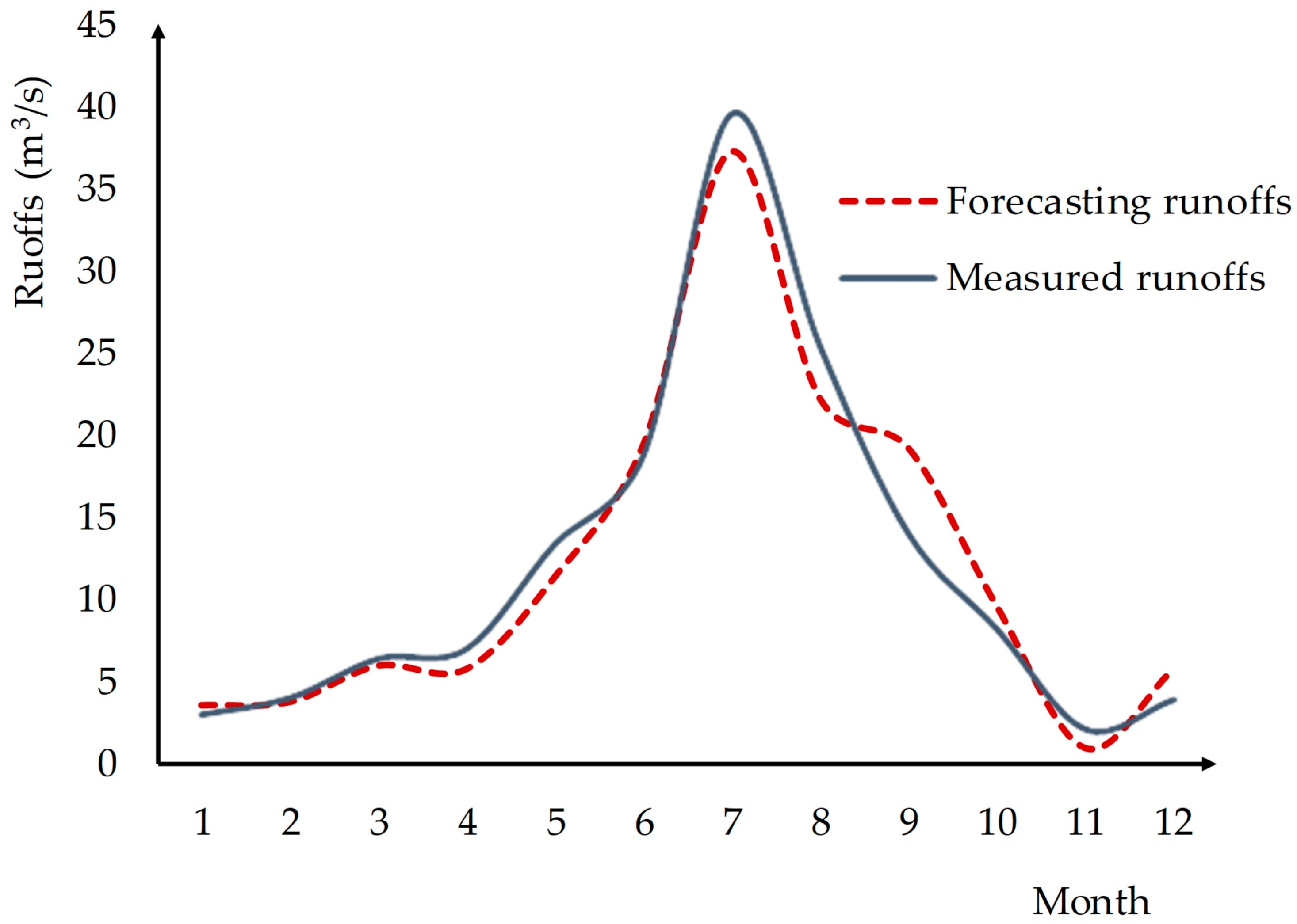
Taking 2003 as an example, according to the prediction model, the calculated periodic wave is extended and linearly superposed to obtain the simulated and predicted values. The comparison of forecasted runoffs results and measured values in 2003 is shown in Figure 3. Table 1 shows the forecasted runoff results in 2003.
Figure 3 and Table 1 indicate that the total forecasted value and measured value are almost the same and the average relative error is 0.20. The application of the periodic mean superposition method in forecasting monthly runoff is effective. In this way, 240 relative error samples of forecasted runoff are obtained. The origin moments of the relative errors are obtained as follows: The first-order origin moment is , the second-order origin moment is , and the third-order origin moment is . The forecasted runoff () in March is m3.
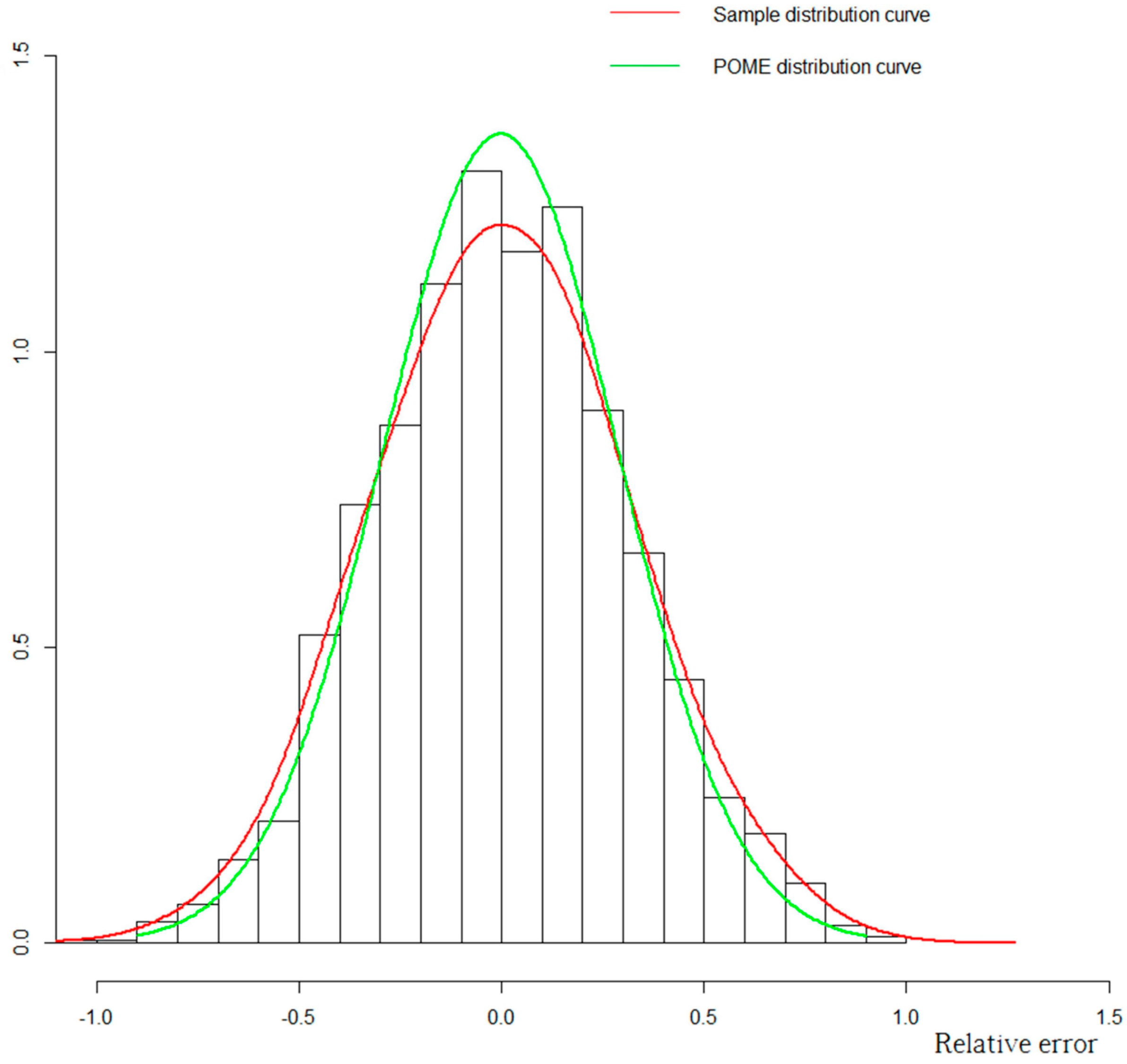
For general engineering problems, the first three order moments can satisfy the precision requirement, so we take as 3 in the maximum entropy model. The Lagrange multipliers can be obtained based on POME: . Therefore, the probability density function of the relative error of forecasted runoffs is
The curve of the is shown in Figure 4, and we also plotted the sample distribution curve. Figure 4 indicates that the distribution curve obtained by POME and the sample distribution are almost the same, and it is reasonable to deduce the probability density function of the relative errors of forecasted runoffs by POME.
Therefore, the probability density function of absolute error of the forecasted runoffs from Equation (9) is
The expected value of the absolute error is , and so the expected runoff () is calculated to be m3.
The total water demand () of the water user in March is m3, and the user chooses to sign a contract with the supply company of the water transfer project; the amount of water purchased through the contract () is m3. The probability density function of the water deficit from Equation (11) is
It is supposed that follows a normal distribution of . The probability density function of is as follows:
3.1.2. Option Trading Model Application and Solution
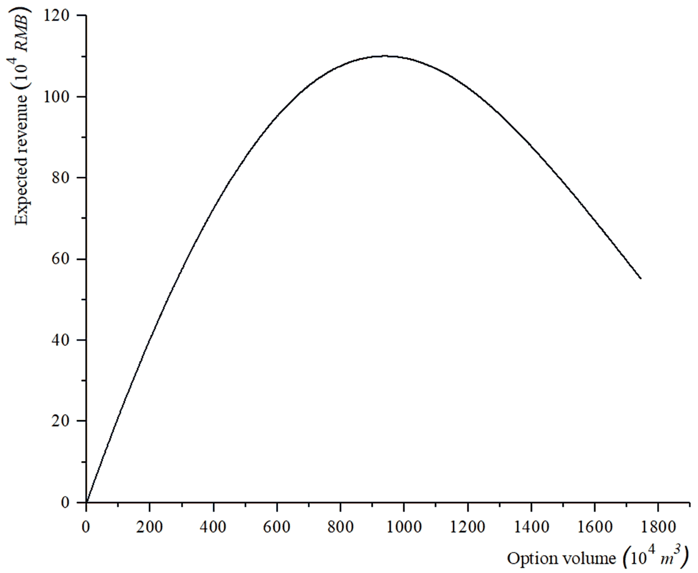
There is an option contract in the options market. We use the calculation method of Section 2.4 to discern Q with a mesh accuracy of m3 into Equation (13) and calculate the series of the expected revenue of the water user (). The graph of the relation between and is as shown in Figure 5: it can be derived from Figure 5 that the expected revenue () is increased first and then decreases as increases. When the pre-purchase volume is m3, the expected revenue of the option is at a maximum of RMB. Therefore, the optimal options trading strategy can help the water users effectively reduce the risk of water shortage caused by the uncertainties of forecasted runoffs and water price.
The optimal solution obtained by the dichotomy method is m3, and accordingly the expected revenue is RMB. The result is consistent with the simulation result described above. Compared with the simulation method, the dichotomy method with the theoretical basis is better, as the simulation method has to discrete the to a certain precision, which will greatly increase the computation time.
3.2. Discussions
Furthermore, different scenarios are set up to explore the effect of the uncertainty degree of local runoff prediction and the spot market price on the optimal options trading volume and the expected revenue of the optimal options .
3.2.1. The Influence of the Uncertainty of the Local Runoff Forecast on the Model
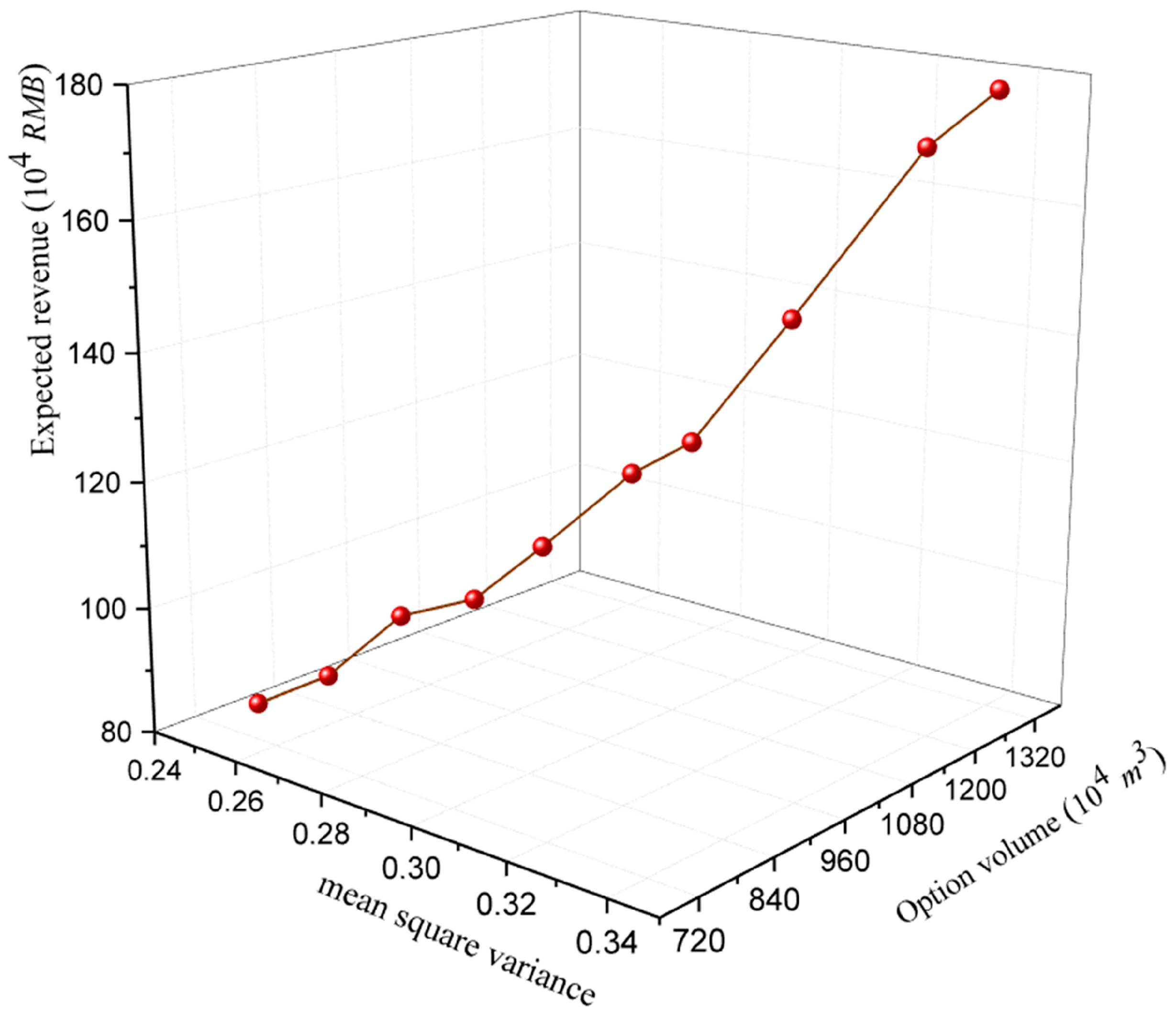
The second-order origin moment of the relative error sample of the forecasted runoffs reflects the uncertainty degree of the forecast runoffs. In order to study the influence of the uncertainty degree of the local runoff forecast on the optimal options trading volume and the expected return of the optimal options, we design experiment scheme 1: change the second-order origin moment of the samples and set other parameters as constants. Table 2 lists the values of other invariant parameters. Then, we use the dichotomy method to find the optimal options trading volume and the expected revenue of the optimal options . Figure 6 is the diagram of the relationship among the mean square variance of samples and the optimal options trading volume and the expected revenue of the optimal options. The results of the experiment scheme 1 are given in Table 3.
The mean variances describe the dispersion degree of random variables around the mean, and the sample mean square variance also reflects the accuracy of the forecast. The smaller the mean square variance is, the more accurate the forecast is; and the larger the mean square variance is, the lower the prediction accuracy is. As shown in Figure 6 and Table 3, the larger the mean deviation is, the larger the optimal options trading volume is. That is because the larger the mean square variance is, the larger the water deficit is, and the more water needs to be purchased through the water option contract to hedge the risk of water shortage due to the shortage of the contract of transferred water. When the mean square variance is small (the forecast accuracy is high), the risk of water shortage is also small, and water users do not need to buy water in large quantities through water options. On the other hand, the larger the mean variance, the greater the revenue the water users can obtain through the optimal water option trading strategy. As a result, the water users are allowed to put a part of the fund into the water option market, and the optimal water option trading strategy can protect the users from the risk of water shortage caused by the uncertainty of local water runoffs.
3.2.2. The Influence of the Fluctuation of Spot Market Price on the Model
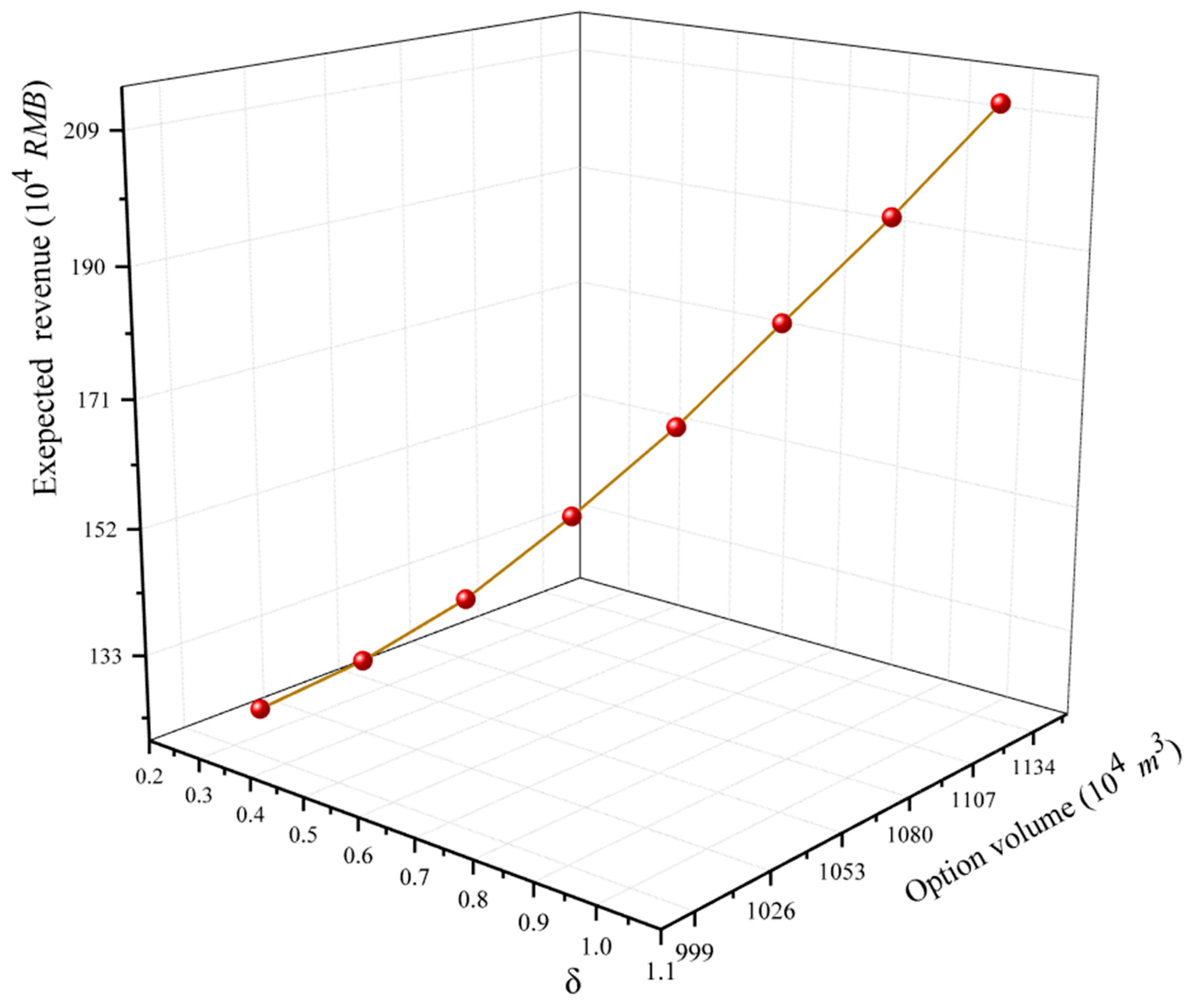
In the same way, to study the effect of the fluctuation of the spot market price on the optimal options trading volume and the expected return of the optimal options, we design experiment scheme 2: vary the values of from 0.3 to 1.0 and set other parameters as constants. Table 4 lists the values of other invariant parameters. Then, we use the dichotomy method to find the optimal options trading volume and the expected return of the optimal options . Figure 7 is the diagram of the relationship among parameter (), the optimal options trading volume and the expected return of the optimal options. Table 5 shows the results of experiment scheme 2.
Parameter () reflects the fluctuation of the spot market price. The greater the value of is, the greater the fluctuation of the spot market price is. It can be concluded from Figure 7 and Table 5 that the optimal option trading volume and the revenue increase with the increase of the value of . That is because the biggest loss of the option is not more than the premium paid for the option, but the water users can yield significant benefits from the sharp fluctuations in the spot market price. Therefore, the water options are purchased with less money, and the optimal water option trading strategy can effectively reduce the risk of high prices caused by the fluctuation of the spot market price.
3.2.3. Application of the Proposed Method
The proposed water option trading model for the uncertainties of water runoff forecasts and the spot market price from the viewpoint of the water users can be applied to the intake area of long-distance water transfer projects. However, this paper only considers a single option and a single user. In future research, we will discuss the decision-making model of water options trading under the coexistence of multi-stakeholders and multiple options. As discussed in Section 2.3 and Section 2.4, the information required to apply the proposed method to the intake area of long-distance water transfer projects include the user’s water demand, forecasted runoffs, forecasted runoff error distribution, the spot market price distribution and option information.
4. Conclusions
In order to solve the risk of water shortages and buying water at high prices caused by the forecasted runoff error and the fluctuation of water price, this paper establishes a water option trading mode, and explores the influence of the water runoff uncertainty and the fluctuation of water price on the water option trading strategy. The main points and conclusions are summarized as follows:
- (1)
- We derived the relative error distribution of forecasted runoffs based on the principle of maximum entropy (POME), and then described the uncertainty of water deficit.
- (2)
- From the perspective of water users, the model of water scarcity risk hedging based on water option trading is established. The dichotomy method was employed to solve the model and to find the optimal water option trading strategy.
- (3)
- The proposed methodology was applied to an intake area of an inter-basin water transfer project in China. Additionally, different scenarios are set up to explore the effect of the uncertainty degree of local runoffs prediction and the spot market price on the optimal options trading volume and the expected revenue of the optimal options .
The results from the case study indicated that the expected revenue () is increased first and then decreases as increases, meaning that there a unique solution to the target function. Therefore, the optimal options trading strategy can help the water users to reduce the risk of water shortage caused by the uncertainties of forecasted runoffs and water price effectively. The optimal options trading volume and the expected revenue () are closely related to the uncertainty degree of local runoff prediction and the spot market price. The optimal options trading volume and the expected revenue () are proportional to the mean square variance of the relative error of the water runoff forecast. As the mean square variance increases, the optimal options trading volume and the expected revenue () increase accordingly. In addition, the greater the fluctuation of the spot market price is, the greater the optimal options trading volume and the expected revenue () are. The proposed model can provide water users with the optimal option strategy and help them to reduce the risk of water shortage caused by the uncertainties of forecasted runoffs and water price effectively.
Author Contributions
This study was carried out through collaboration among all authors. H.Y. and P.Z. conceived and designed the experiments; H.Y. and J.C. performed the experiments; B.X. and Y.W. contributed to the results and discussion; Y.W. and F.Z. analyzed the data. H.Y. and J.C. wrote the paper. All authors read and approved the final manuscript.
Funding
This research was funded by the National Key R&D Program of China under Grant No. 2017YFC0405606, the National Natural Science Foundation of China under Grant No. 51579068, the Fundamental Funds for the Central Universities under Grant No. 2018B18214 and the China Postdoctoral Science Foundation under Grant No. 2017M621612.
Conflicts of Interest
The authors declare no conflict of interest.
References
- Kumar, A.; Sharma, M.P. Assessment of risk of GHG emissions from Tehri hydropower reservoir, India. Hum. Ecol. Risk Assess. Int. J. 2016, 22, 71–85. [Google Scholar] [CrossRef]
- You, J.J.; Wang, Z.J.; Gan, H.; Jiang, Y.Z. Current status and prospect of study in china on water allocation of inter-basin diversion projects. South North Water Transf. Water Sci. Technol. 2008, 3, 6. [Google Scholar]
- Zhong, P.; Wang, H.; Liu, J.; Chen, X.; Chen, K. Optimal dispatching model for Shenzhen water resources system. J. Hehai Univ. 2003, 31, 616–620. [Google Scholar]
- Chen, J.; Zhong, P.A.; Xu, B.; Zhao, Y.F. Risk analysis for real-time flood control operation of a reservoir. J. Water Resour. Plan. Manag. 2015, 141, 04014092. [Google Scholar] [CrossRef]
- Zhu, F.; Zhong, P.A.; Sun, Y.; Yeh, W.W.G. Real-time optimal flood control decision making and risk propagation under multiple uncertainties. Water Resour. Res. 2017, 53, 10635–10654. [Google Scholar] [CrossRef]
- Antonelli, M.; Tamea, S. Food-water security and virtual water trade in the middle east and North Africa. Int. J. Water Resour. Dev. 2015, 31, 326–342. [Google Scholar] [CrossRef]
- Grafton, R.Q.; Landry, C.; Libecap, G.D.; Mcglennon, S.; O’Brien, R. An integrated assessment of water markets: Australia, Chile, China, South Africa and the USA. Cent. Water Econ. Environ. Policy Pap. 2010, 5. [Google Scholar] [CrossRef]
- Fu, J.; Zhong, P.A.; Zhu, F.; Chen, J.; Wu, Y.N.; Xu, B. Water resources allocation in transboundary river based on asymmetric Nash–Harsanyi Leader–Follower game model. Water 2018, 10, 270. [Google Scholar] [CrossRef]
- Ha, M.; Gao, Z. Optimization of water allocation decisions under uncertainty: The case of option contracts. J. Ambient. Intell. Humaniz. Comput. 2017, 8, 809–818. [Google Scholar] [CrossRef]
- Brookshire, D.S.; Ganderton, P.T. Introduction to special section on water markets and banking: Institutional evolution and empirical perspectives. Water Resour. Res. 2004, 40, 547. [Google Scholar] [CrossRef]
- Jercich, S.A. California’s 1995 water bank program: Purchasing water supply options. J. Water Resour. Plan. Manag. 1997, 123, 59–65. [Google Scholar] [CrossRef]
- Calatrava, J.; Garrido, A. Spot water markets and risk in water supply. Agric. Econ. 2015, 33, 131–143. [Google Scholar] [CrossRef]
- Porkka, M.; Kummu, M.; Siebert, S.; Florke, M. The role of virtual water flows in physical water scarcity: The case of central Asia. Int. J. Water Resour. Dev. 2012, 28, 453–474. [Google Scholar] [CrossRef]
- Wichelns, D. Virtual water and water footprints offer limited insight regarding important policy questions. Int. J. Water Resour. Dev. 2010, 26, 639–651. [Google Scholar] [CrossRef]
- Hansen, K.; Kaplan, J.; Kroll, S. Valuing options in water markets: A laboratory investigation. Environ. Resour. Econ. 2014, 57, 59–80. [Google Scholar] [CrossRef]
- Hansen, K.; Williams, J. Valuing risk: Options in California water markets. Am. J. Agric. Econ. 2010, 90, 1336–1342. [Google Scholar] [CrossRef]
- Cheng, W.C.; Hsu, N.S.; Cheng, W.M.; Yeh, W.W.G. Optimization of European call options considering physical delivery network and reservoir operation rules. Water Resour. Res. 2011, 47. [Google Scholar] [CrossRef] [Green Version]
- Tomkins, C.D.; Weber, T.A. Option contracting in the California water market. J. Regul. Econ. 2010, 37, 107–141. [Google Scholar] [CrossRef]
- Rey, D.; Calatrava, J.; Garrido, A. Optimisation of water procurement decisions in an irrigation district: The role of option contracts. Aust. J. Agric. Resour. Econ. 2016, 60, 1–25. [Google Scholar] [CrossRef]
- Kasprzyk, J.R.; Reed, P.M.; Kirsch, B.R.; Characklis, G.W. Managing population and drought risks using many-objective water portfolio planning under uncertainty. Water Resour. Res. 2009, 45, 170. [Google Scholar] [CrossRef]
- Cui, J.; Schreider, S. Modelling of pricing and market impacts for water options. J. Hydrol. 2009, 371, 31–41. [Google Scholar] [CrossRef]
- Holburt, M.B.; Atwater, R.W.; Quinn, T.H. Water marketing in southern California. J. Am. Water Works Assoc. 1988, 80, 38–45. [Google Scholar] [CrossRef]
- Michelsen, A.M.; Young, R.A. Optioning agricultural water rights for urban water supplies during drought. Am. J. Agric. Econ. 1993, 75, 1010–1020. [Google Scholar] [CrossRef]
- Mudança Climática. Climate Change Adaptation: The Pivotal Role of Water; UN-Water: Ginebra, Suiza, 2010. [Google Scholar]
- Villinski, M.T. A numerical quadrature approach to option valuation in water markets. Am. Agric. Econ. Assoc. 1999, 81, 1321. [Google Scholar]
- Ramos, A.G.; Garrido, A. Formal risk-transfer mechanisms for allocating uncertain water resources: The case of option contracts. Water Resour. Res. 2004, 40, 73–74. [Google Scholar]
- Ranjan, R. Factors affecting participation in spot and options markets for water. J. Water Resour. Plan. Manag. 2004, 136, 454–462. [Google Scholar] [CrossRef]
- Diao, Y.F.; Wang, B.D.; Liu, J. Study on distribution of flood forecasting errors by the method based on maximum entropy. J. Hydraul. Eng. 2007, 38, 591–595. [Google Scholar]
- Wheeler, S.; Bjornlund, H.; Shanahan, M.; Zuo, A. Price elasticity of water allocations demand in the goulburn–murray irrigation district. Aust. J. Agric. Resour. Econ. 2010, 52, 37–55. [Google Scholar] [CrossRef]
- Wuab, D.J.; Zhang, J.E. Optimal bidding and contracting strategies for capital-intensive goods. Eur. J. Oper. Res. 2002, 137, 657–676. [Google Scholar]
Figure 1.
Two-stage water option trading decision model flow chart.

Figure 2.
Schematic diagram deriving the method of relative error distribution of the forecasted runoffs. (a) Scatter plot of relative error; (b) frequency histogram of relative error; (c) principle of maximum entropy distribution curve.
Figure 2.
Schematic diagram deriving the method of relative error distribution of the forecasted runoffs. (a) Scatter plot of relative error; (b) frequency histogram of relative error; (c) principle of maximum entropy distribution curve.

Figure 3.
Comparison of forecasted runoff results and measured values.

Figure 4.
Comparison of the principle of maximum entropy (POME) distribution curve and the sample distribution curve.
Figure 4.
Comparison of the principle of maximum entropy (POME) distribution curve and the sample distribution curve.

Figure 5.
The relation curve between the amount of option trading and the expected revenue.

Figure 6.
The relationship among the mean square variance, the optimal options trading volume and the expected revenue of the optimal options.
Figure 6.
The relationship among the mean square variance, the optimal options trading volume and the expected revenue of the optimal options.

Figure 7.
The relationship among parameter ( ), the optimal options trading volume and the expected return of the optimal options.
Figure 7.
The relationship among parameter ( ), the optimal options trading volume and the expected return of the optimal options.


Table 1.
Statistical analysis table of forecasted runoff results in 2003.
| Forecast Period | Forecasting Runoffs (m3/s) | Measured Runoffs (m3/s) | Absolute Error (m3/s) | Relative Error |
|---|---|---|---|---|
| January | 3.6 | 3 | −0.6 | −0.2 |
| February | 3.8 | 4 | 0.2 | 0.05 |
| March | 6 | 6.4 | 0.4 | 0.06 |
| April | 5.8 | 7 | 1.2 | 0.17 |
| May | 11.4 | 13.4 | 2 | 0.15 |
| June | 19.4 | 18.8 | −0.6 | −0.03 |
| July | 37.2 | 39.6 | 2.4 | 0.06 |
| August | 22.2 | 25.4 | 3.2 | 0.13 |
| September | 19.2 | 14 | −5.2 | −0.37 |
| October | 9.6 | 8.2 | −1.4 | −0.17 |
| November | 1 | 2.1 | 1.1 | 0.52 |
| December | 5.8 | 3.9 | −1.9 | −0.49 |
| Average | 12.1 | 12.2 | 0.1 | 0.20 |
Table 2.
Model parameters of experiment scheme 1.
| W (104 m3) | β1 (104 RMB) | β2 (104 RMB) | μ | δ | m1 | m3 |
|---|---|---|---|---|---|---|
| 3000 | 2 | 0.1 | 2.5 | 0.3 | 0.00116156 | 0.000219 |
Table 3.
The results of experiment scheme 1.
| m2 | 0.25 | 0.26 | 0.27 | 0.28 | 0.29 | 0.3 | 0.31 | 0.32 | 0.33 | 0.34 |
|---|---|---|---|---|---|---|---|---|---|---|
| Q* (104 m3) | 755 | 800 | 849 | 897 | 936 | 1008 | 1029 | 1115 | 1263 | 1299 |
| N (104 RMB) | 83 | 88 | 98 | 101 | 110 | 121 | 127 | 145 | 169 | 178 |
Table 4.
Model parameters of experiment scheme 2.
| W (104 m3) | β1 (104 RMB) | β2 (104 RMB) | μ | λ0 | λ1 | λ2 | λ3 |
|---|---|---|---|---|---|---|---|
| 3000 | 2 | 0.1 | 2.5 | 0.3133 | −0.0326 | −5.879 | −0.0136 |
Table 5.
The results of experiment scheme 2.
| m2 | 0.3 | 0.4 | 0.5 | 0.6 | 0.7 | 0.8 | 0.9 | 1 |
|---|---|---|---|---|---|---|---|---|
| Q* (104 m3) | 1008 | 1026 | 1044 | 1063 | 1081 | 1099 | 1118 | 1136 |
| N (104 RMB) | 124 | 131 | 140 | 152 | 165 | 180 | 195 | 211 |
© 2018 by the authors. Licensee MDPI, Basel, Switzerland. This article is an open access article distributed under the terms and conditions of the Creative Commons Attribution (CC BY) license (http://creativecommons.org/licenses/by/4.0/).
Share and Cite
MDPI and ACS Style
Yan, H.; Zhong, P.-A.; Chen, J.; Xu, B.; Wu, Y.; Zhu, F. An Optimal Model for Water Resources Risk Hedging Based on Water Option Trading. Water 2018, 10, 1026. https://doi.org/10.3390/w10081026
AMA Style
Yan H, Zhong P-A, Chen J, Xu B, Wu Y, Zhu F. An Optimal Model for Water Resources Risk Hedging Based on Water Option Trading. Water. 2018; 10(8):1026. https://doi.org/10.3390/w10081026
Chicago/Turabian StyleYan, Haibin, Ping-An Zhong, Juan Chen, Bin Xu, Yenan Wu, and Feilin Zhu. 2018. "An Optimal Model for Water Resources Risk Hedging Based on Water Option Trading" Water 10, no. 8: 1026. https://doi.org/10.3390/w10081026
Note that from the first issue of 2016, this journal uses article numbers instead of page numbers. See further details here.