Combination of Measurement Methods for a Wide-Range Description of Hydraulic Soil Properties

Abstract

Established measurement methods for hydraulic soil properties cover a limited soil moisture range. Simulations of soil water dynamics based on such observations are therefore rarely representative for all conditions from saturation to drought. Recent technical developments facilitate efficient and cheap collecting of soil water characteristics data, but the quantitative benefit of extended measurement campaigns has not been adequately tested yet. In this study, a combination of four methods to measure water retention and hydraulic conductivity at different moisture ranges was applied. Evaporation method, dewpoint psychrometry, hood infiltrometer experiments, and falling head method for saturated conductivity were conducted at two experimental sites in eastern Austria. Effects of including the particular methods in the measurement strategy were examined by visual evaluation and a 1D-modelling sensitivity study including drainage, infiltration and drought conditions. The evaporation method was considered essential due to its broad measurement range both for water retention and hydraulic conductivity. In addition to that, the highest effect on simulated water balance components was induced by the inclusion of separate conductivity measurements near saturation. Water content after three days of drainage was 15 percent higher and the transpiration rate in a drought period was 22 percent higher without near-saturated conductivity measurements. Based on relative comparisons between different combinations, we suggested combining evaporation method and hood infiltrometer experiments as the basis for representative predictions of soil water dynamics.

1. Introduction

Numerical simulations of soil water dynamics are supposed to comprise a wide range of soil moisture conditions; matching simulation data with reality is a fundamental issue of soil science [1,2]. The components which control a model’s ability to represent reality over the full moisture range are the hydraulic soil properties (HSP). In most modelling applications, HSP are formalized in two mathematical functions: (i) the water retention function $\theta (h)$, the relation of volumetric soil water content $\theta$ and soil water head h; and (ii) the hydraulic conductivity function $K(h)$, where K is the hydraulic conductivity of soil [1,3]. These functions are defined by parameters which may be derived indirectly by empirical pedotransfer functions (PTF) [4,5] or from direct measurements of $\theta (h)$ and $K(h)$ [6].

In contrast to PTF, direct measurements of HSP allow for site-specific capture of soil physical characteristics with high spatial and temporal resolution. Most of the established direct measurement methods yield data only for the retention function or for a limited range of soil moisture [7,8]. Furthermore, HSP-parameters are often obtained from fits to the retention curve and the corresponding conductivity curve is scaled by a single measured value, the saturated conductivity (e.g., [9]). Consequently, shape information of $K(h)$ is neglected. Extensive overviews of options to determine HSP were presented before [6]. One of the most established methods is a multi-step outflow experiment, where a sequence of positive pressure values is applied to a soil sample and water content and outflow is recorded. Depending on the actual setup, measurements near saturation (h = 0 to −10 cm) and at dry conditions (h < −1000 cm) are hardly possible or very time consuming. The same principle is applied in hanging water column, pressure cell or sand box experiments. Their setup is simpler, but the ranges of measurements are even narrower [6]. Multi-step outflow experiments are also done in centrifuges. A sequence of water heads is applied via rotation and centrifugal force and water content and outflow rates are measured [10,11]. This approach has been continuously developed to eliminate practical issues like consolidation of undisturbed samples [12]. In addition, the evaporation method [13] is widely used, which allows high-resolution observation of HSP from saturation (only retention curve) to around h = −1000 cm and in an extended version up to h = −8800 cm [14]. In the field, the instantaneous profile approach describes various types of soil profiles equipped with sensors for water content and soil water head in at least two depths [15]. The importance of this method is small due to its high demands on equipment and logistics.

A major part of actual studies calls for a sounder data basis for the parametrization of HSP, especially concerning the range of represented soil moisture and the sampled soil volume (e.g., [16,17]). Additionally, simultaneous determination of $\theta (h)$ and $K(h)$ is desired to use the full capacity of wide-range measurements of both HSP-functions [7]. For such simultaneous determination, two general approaches are used: (i) recordings of a water flow process and subsequent inverse modelling; and (ii) fitting of HSP-functions to measured data of $\theta (h)$ and $K(h)$. Exemplary observation setups for (i) are: one- or multistep outflow lab experiments (e.g., [18,19]), evaporation experiments [20], infiltration experiments in the field [17,21,22], or field monitoring of soil water state [23,24]. Inverse modelling rapidly gives reliable results and is the most established method to obtain HSP. Nevertheless, reference observations are needed which require considerable time or equipment resources, especially in field-based studies.

In contrast to inverse simulation, wide-moisture-range measurement of data for both HSP-functions with subsequent direct fitting is rarely done. Multi-step flux experiments are advancements of multi-step outflow methods and allow to measure HSP directly in disturbed samples [25,26]. Peters and Durner [27] used virtual evaporation experiments as the data basis for simultaneous HSP-fitting, interpreted their results as reliable and pointed out the need for additional information in $K(h)$ near saturation. The intention of their study was to test models, not to evaluate measurement methods. In a comparative study, Mermoud and Xu [28] obtained HSP-parameters from direct field and lab measurements as well as by using four PTF. By modelling they examined which results are most appropriate to reproduce field-observed water content. They found best agreement with HSP from field measurements, less quality with lab experiments and poor results with PTF. Their field experiments were intensively equipped and laborious and the data analysis was done for each method separately. A combination of methods in the parametrization procedure might allow a reduction of effort in field measurements. Siltecho et al. [29] also compared different approaches including rapid and cheap field and lab measurements, PTF and inverse modelling. No method was found to be superior and they suggested the use of the cheapest and easiest method to obtain starting values for a more elaborate inverse parametrization or model calibration.

To establish statements about the appropriateness of different HSP-parametrization approaches, measures for the goodness of fits are usually used [30]. They allow a statement about the alignment of reference values to a simplifying model. Nevertheless, information about the representation of natural water dynamics or the effects of changing options in the measuring-fitting procedure may be only gained by subsequent modelling. Such functional approaches were applied to evaluate effectivity of uni- or bimodal soil hydraulic characterization [31], to compare the ability of different models to account for dry periods [32] or to evaluate different PTF [33].

In summary, the potential of combining methods, preferably field and lab experiments, to yield a comprehensive data basis for the parametrization of HSP was repeatedly pointed out. Nevertheless, there are few studies which conclusively suggest an optimum strategy for HSP measurements due to high experimental efforts with uncertain benefit. There is a need to develop and evaluate methods to measure data over a wide range of soil moisture states. Especially for studies on field- or catchment scale, rapid and cheap technologies are required which allow a high number of replications to capture a possibly representative soil volume. The aim of this study was to show if combining multiple methods for acquisition of HSP-data is an efficient strategy to subsequently obtain reliable results in modelling applications.

2. Materials and Methods

2.1. Summary of Methodology

Four rapid methods were applied to measure HSP: (i) the evaporation method (EM) [14]; (ii) a dew point hygrometer [34]; (iii) the falling head method for saturated hydraulic conductivity [35], and (iv) the hood infiltrometer (HI), a type of tension infiltrometer [36]. The widely used bimodal HSP-functions of Priesack and Durner [37], based on van Genuchten [38] and Mualem [39], were fitted simultaneously to different combinations of measured data. To evaluate the measurements, we used a functional approach [31] and conducted a numerical sensitivity study including drainage, infiltration, and drying conditions. This allowed to estimate quantitatively how different measurement methods alter soil water balance. Additionally, we discussed characteristics of used methods concerning application issues and reliability.

2.2. Sampling Sites and Procedure

Experiments and soil sampling were carried out at two long-term tillage experiments in north-eastern Austria (

Table 1. Study site description. Grain size distribution classified as: 2 mm ≥ sand > 0.063 mm ≥ silt > 0.002 mm ≥ clay [41]. Coordinates refer to the Universal Transverse Mercator system (UTM), zone 33N.

	Site A	Site B
location name	Obersiebenbrunn	Hollabrunn
crop	winter wheat	sunflower
sand	34%	24%
silt	50%	55%
clay	16%	21%
soil type	Chernozem	Chernozem
mean annual precipitation	520 mm	519 mm
soil organic carbon	1–2%	1–2%
coordinates field site	E 625720, N 5347520	E 578580, N 5379390
coordinates weather station	E 625992, N 5347056	E 578953, N 5380331
measurement dates 2016	02, 05, and 06 May	13, 14, and 16 June

). In each soil unit (defined by same site and tillage treatment), measurements and sampling were replicated 11 times (

Table 2. Number of replicates per analysed unit. T1 to T4 are different tillage treatments (not in the focus of this study, hence not explained).

Treatments	Sites
	Site A	Site B
T1	11	11
T2	11	11
T3	11	12
T4	11	10

, values 10 and 12 resulted from a mapping error). Sampling positions were predetermined on a 6 × 12 m raster and placed in inter-row space avoiding machine tracks. The measurements were carried out in early summer when soil water status was neither around saturation nor drying cracks were present on the soil surface (i.e., vol. water content $\theta$ = 0.20 to 0.35 cm³ cm⁻³). At sampling time, plant cover was established over the whole field area, minimizing structural degradation like crusting, shrinking or splash erosion. Fraction of stable soil aggregates (measured after Kemper and Koch [40]) ranged from 0.15 to 0.5 with a median at 0.31 depending on site and tillage treatment. Similarly, macro-porous soil structure development was considerably variable as visual estimation showed. This plurality was appreciated to account for a majority of possible conditions of agricultural soils in the study region.

2.3. Field and Lab Measurement Methods

To measure hydraulic soil properties, four methods were applied sequentially to the same soil sample. The field measurement procedure included the following steps:

(i)

hood infiltrometer experiment, see Section 2.3—HI;

(ii)

percolation and drying time, at least 2 h, to minimize soil smearing during subsequent sampling;

(iii)

soil core sampling, one ring placed at the centre of the infiltration area from (i), carefully pushed in without hammering to avoid sample disturbance or tilting, steel rings with inner diameter $d_{in}=84$ mm and height $h=50$ mm, another ring in a distance of approximately one meter for measurement of initial water content and as backup sample;

(iv)

collecting disturbed soil samples (ca. 500 cm³) from the immediate surroundings of the core.

The methods are listed below and each of them yields data at a certain range of soil moisture state (Figure 1). During all measurements, soil water head decreased to more negative, which means we nominally measured drainage conditions to avoid bias due to hysteresis. Still, the infiltration observed with the HI may also be considered as wetting process. Consequently, measurements of HI and EM (draining process) could not be combined. Nevertheless, hysteresis in tension infiltrometer measurements is present, but does not impact quantitative outcomes in application cases [42,43]. As the HI additionally yields data for a very narrow range of h near saturation, where hysteresis in HSP is minimal, hysteresis was negligible in this study setup. To determine bulk density for calculation of volumetric water content $\theta$, sample rings were dried after the experiments at 105 °C for 24 h. As the samples were taken a few hours after infiltration experiments, bulk density corresponds to conditions near field capacity.

HI Hood Infiltrometer

The hood infiltrometer [36] is a type of tension infiltrometer which lets water infiltrate into the soil directly from an open-bottomed, semi-spheric hood without any artificial contact layer. Via a connected Mariotte bottle system, tension is established which has to be overcome by the soil matrix to initiate infiltration. The achievable minimum water head is restricted by entrance of air from soil into the water-filled hood, which usually occurred at around h = −3 cm in this study (range ca. −1.5 to −7 cm).

To prepare the measurement, a level area in the micro-relief was chosen where loose plant and soil clod material was carefully removed. After installing the infiltrometer hood, the first tension step was set at approximately $h=-0.5$ cm and infiltration started for a few minutes without measuring to initially wet the soil body. Tension was kept constant until a steady infiltration rate for at least 3 min was reached (reading time steps were 15 to 60 s). Subsequently, two further pressure steps were measured, one around $h=-2$ cm and the last one slightly less negative than air entry pressure. As a result, three data points for near-saturated hydraulic conductivity are derived from the infiltration rate. Calculation of $K(h_i)$ from readings of water outflow $Q_i$ (in cm³ s⁻¹) and water head $h_i$ followed the suggested procedure in Schwärzel and Punzel [36].

FH Falling Head Method

Saturated hydraulic conductivity $K_s$ was measured directly in undisturbed soil core samples by the falling head method with rising water level [44], modified after Klute and Dirksen [35]. As a simplification for further analysis, the corresponding water head for $K_s$ was nominally set to h = −0.01 cm (pF = −2).

EM Evaporation Method

Undisturbed soil cores were placed on a digital measuring device (HYPROP^® METER Group AG, Munich, Germany; cf. Schindler et al. [14] for details). Two tensiometers measure the water head h in different depths and water content $\theta$ is determined by weighing. Additionally, the measurement range was extended to the tensiometer’s air-entry point at h = −8800 cm [14]. Measured data were transformed to data points at the retention curve $\theta (h)$ (range: h = 0 to −8800 cm) and the hydraulic conductivity curve $K(h)$ (range: h = ca. −20 to −8800 cm). The experiments were run in a lab at a temperature of 21–23 °C and air humidity of 20–40%.

DP Dew Point Method

A dew point hygrometer (WP4C PotentiaMeter^® METER Group AG, Munich, Germany) was used to measure water retention $\theta (h)$ under dry conditions (pF = 3.5–6.2). Here, the liquid water phase in the soil sample and the vapour phase in surrounding air is equilibrated in a sealed chamber. Finally, water potentials of vapour and liquid phase are equal and the former is measured via the dew point on a cooled mirror inside of the chamber. A detailed description of the measurement principle is given elsewhere [34,45]. Water content for each reading is measured gravimetrically and transformed to volumetric $\theta$ via the average bulk density of the corresponding EM-cores. Before DP-measurements, samples of the same treatments were mixed and two replicates of the mixed samples were analysed. 3–4 g of air-dry soil was put into circular steel cups (d = 37 mm) and wetted using deionized water to around $\theta$ = 0.2 cm³ cm⁻³. During air drying the sample, up to seven measurements in precise mode—repeated readings until they remain within a defined level of tolerance—were taken of each sample with the intention to obtain values evenly distributed between pF = 3.5 and 6.2.

For further analysis, six combinations of measurement methods were defined and compared. Only EM was included in all combinations. It serves as the backbone method due to its wide measuring range at both HSP-curves. Data from all other methods were variably omitted and the following combinations were analysed: ALL, EM + FH + HI, EM + FH, EM + HI, EM + DP, EM.

2.4. Fitting of Functions for Hydraulic Soil Properties

For the formalization of HSP, we used the van Genuchten-Mualem model (VGM) [38,39] in its bimodal version (Equations (1)–(3) [37]). This model was chosen because of its high acceptance and its compatibility to the later used modelling software HYDRUS-1D (PC-Progress, Prague, Czech Republic) [46]. The bimodal version superimposes two subcurves to be able to account for two different flow domains in soil, usually macropore system and soil matrix. In this case, a pre-study comparing goodness of fit for uni- and bimodal model did not show significant differences. Nevertheless, the bimodal model was used to enable usage of the approach also for highly structured soils.

Introduced variables and parameters in VGM are: ${\theta }_s$ is the volumetric water content at saturation (cm³ cm⁻³), $S_e$ is the degree of saturation ($S_e=\theta /{\theta }_s$, dimensionless), $\alpha$ (cm⁻¹, commonly denoted as reciprocal of the air-entry point of soil), n, and $\tau$ (both dimensionless, parameter defining the slope of the retention curve and tortuosity parameter, respectively) are fitting parameters of VGM, J is the number of subcurves in the used model (i.e., $J=1$ for uni-modal and $J=2$ for bi-modal functions), w is a dimensionless weighing factor for the respective subcurve j. Herein, the index j = 1 always relates to the subcurve for the flow domain comprising the coarser pores (i.e., ${\alpha }_1$ > ${\alpha }_2$). Furthermore, we used a simplified form with residual water content ${\theta }_r=0$ and $m=1-1/n$.

$$\theta (h)=({\theta }_s-{\theta }_r)S_e(h)$$

(1)

$$S_e(h)=\sum _{j=1}^J{w}_j{\left[1+{({\alpha }_{j}h)}^{n_j}\right]}^{-m_j}$$

(2)

$$K(h)=K_s{\left(\sum _{j=1}^J{w}_j{\left[1+{({\alpha }_{j}h)}^{n_j}\right]}^{-m_j}\right)}^{\tau }{\left({\displaystyle \frac{{\sum }_{j=1}^J{w}_j{\alpha }_j\{1-{\left({\alpha }_{j}h\right)}^{n_j}{\left[1+{({\alpha }_{j}h)}^{n_j}\right]}^{-m_j}\}}{{\sum }_{j=1}^J{w}_j{\alpha }_j}}\right)}^2$$

(3)

The functions $\theta (h)$ and $K(h)$ (Equations (1)–(3)) were fitted simultaneously to measured data by use of the artificial bee colony global optimization algorithm ([47], implemented in [48]) minimizing the objective function given in Equation (4). There, $\mathsf{\Phi }$ is the evaluation criterion to be minimized, r and k are the number of observations in the respective data class, $\mathit{b}$ is the parameter vector, hence $\widehat{{\theta }_i}(\mathit{b})$ and $\widehat{K_i}(\mathit{b})$ are model predicted values and $\overline{{\theta }_i}$ and $\overline{K_i}$ are measurements. The weighting factor of 0.5 for the conductivity curve in Equation (4) was based on a pre-study (unpublished) using a representative part of the dataset. Additionally, ranges for the parameters were predestined according to literature [9,49,50] and visual plausibility evaluations (

Table 3. Boundaries for parameters of bimodal van Genuchten-Mualem model. Parameters are: ${\alpha }_j$ in cm⁻¹, $n_j$ and $\tau$, both dimensionless, are fitting parameters; ${\theta }_s$, in cm³ cm⁻³, is saturated water content; $w_2$, dimensionless, is the weight of the second sub-function; and $K_s$ in cm day⁻¹ is saturated hydraulic conductivity.

Parameter	${\mathit{\theta }}_{\mathit{s}}$	${\mathit{\alpha }}_{\mathbf{1}}$	${\mathit{n}}_{\mathbf{1}}$	${\mathit{\alpha }}_{\mathbf{2}}$	${\mathit{n}}_{\mathbf{2}}$	${\mathit{w}}_{\mathbf{2}}$	${\mathit{K}}_{\mathit{s}}$	$\mathit{\tau }$
upper boundary	1	0.5	15	0.5	15	1	${10}^5$	10
lower boundary	0.1	10−5	1.01	10−5	1.01	0	1	−2

). For the physically related parameters ${\theta }_s$ and $K_s$, information from measurements was also used.

$$\mathsf{\Phi }(\mathit{b})=\sum _{i=1}^r{\left[\overline{{\theta }_i}-\widehat{{\theta }_i}(\mathit{b})\right]}^2+0.5\sum _{i=1}^k{\left[{\log }_{10}(\overline{K_i})-{\log }_{10}(\widehat{K_i})(\mathit{b})\right]}^2$$

(4)

2.5. Numerical Simulations

A three-part sensitivity study using HYDRUS-1D [46] was run to assess the effects of different method combinations on soil water balance components. The setup was adopted from Romano and Nasta [31] and includes a drainage, an infiltration, and a drying process. Accordingly, simulations were conducted without accounting for hysteresis considering the arguments given in Section 2.3. Nevertheless, for the infiltration experiment, HSP during wetting are decisive and hysteresis would have an effect. Consequently, the infiltration experiment will be interpreted with caution to potential bias due to neglected hysteresis.

For all simulations, we defined a soil column of 200 cm depth but analysis comprised only the soil region from z = 0–50 cm. The soil material was constant all over depth and its HSP were determined by the different combinations of measurements following the procedure in Section 2.4. Separate model runs were conducted for each sample and measurement combination (528 runs, see Section 2.6). The drainage process started at fully saturated state (h = 0 cm) and ran for 72 h with zero flux as top boundary condition and free drainage at the bottom. The vertical distribution of water head after the drainage simulation was taken as initial condition for the infiltration experiment. Therein, boundary conditions were set to a constant water head of h = 0 cm at the top and free drainage at bottom. The infiltration simulation was run for 24 h.

The drying process started with a global initial water head of h = −100 cm and was simulated for 45 days. Boundary conditions were free drainage at the bottom and an atmospheric top with zero precipitation and constant rates of potential evaporation (2 mm day⁻¹) and potential transpiration (7.5 mm day⁻¹). These rates represent high but plausible summer values for the sampling regions. We defined a grass vegetation cover with a constant height of 12 cm and rooting depth of 50 cm (water uptake was equally distributed from z = 0–50 cm). Hence, the difference between actual and potential transpiration was exclusively determined by HSP. The water stress response function after Feddes [51] was applied with standard parameters for grass [46].

2.6. Data Processing and Statistics

The measurement procedure was applied at 88 soil sampling units (Table 2). In the calculations, each was described with six combinations of measurement methods, what leads to 528 data sets. The fitting procedure (Section 2.4) was applied to each data set resulting in a set of parameters as input for a separate model run. Results of the modelling study were normalized by the corresponding value of ALL to eliminate the influence of treatment and site as disturbing factors. More in detail, the presented numbers (Section 3.2) were calculated in three steps: (i) averaging replicate results for identical site, treatment and method combination (from 528 to 48 values); (ii) divide these by the result from ALL on the same site and same tillage treatment (48 absolute to 48 relative values); (iii) calculate average of relative values for each combination of measurement methods (48 to 6).

For all data processing we used the statistical software environment R, version 3.3.1 [52]. Differences between results for data units were detected by ANOVA, Tukey’s HSD-test [53] was used as post-hoc test to define coherent groups [54]. Data sets for $\theta (h)$ and $K(h)$ will be provided as supplementary material.

3. Results

3.1. Fitting of HSP-Functions

Goodness of fits may be estimated visually in Figure 2. The values for ${\theta }_{sim}$ and $K_{sim}$ were calculated for all measured values of h (combination ALL) using Equations (1)–(3). Irregular patterns occurred in both combinations without measurements for (near-)saturated conductivity: EM and EM + DP (subsequently denoted as NoCon). In contrast, all other combinations (subsequently denoted as YesCon) gave a good overall picture without a systematic pattern of deviations. The methods FH and HI represented the near-saturated conductivity curve, where FH induces higher variability (Figure 1 and Figure 2).

Table 4. Fitted parameters of bimodal van Genuchten-Mualem model and evaluation criterion root mean square error (RMSE).

		ALL	EM + FH + HI	EM + FH	EM + HI	EM + DP	EM
${\log }_{10}(K_s$/cm ${\mathrm{day}}^{-1})$	mean (sd)	2.50 (0.61)	2.55 (0.62)	2.39 (0.90)	2.35 (0.59)	0.10 (0.26)	0.11 (0.28)
	min–max	0.99–3.61	1.12–4.08	0.00–4.11	1.14–3.75	−0.75–0.44	−0.86–0.46
${\theta }_s$/cm3 cm−3	mean (sd)	0.48 (0.04)	0.48 (0.04)	0.48 (0.04)	0.48 (0.04)	0.45 (0.03)	0.45 (0.03)
	min–max	0.41–0.62	0.41–0.61	0.40–0.62	0.42–0.62	0.39–0.59	0.39–0.57
${\log }_{10}({\alpha }_1$/${\mathrm{cm}}^{-1})$	mean (sd)	−0.9 (0.5)	−0.9 (0.4)	−0.9 (0.5)	−1.0 (0.5)	−1.8 (0.4)	−1.8 (0.4)
	min–max	−1.8–−0.3	−1.9–−0.3	−2.1–−0.3	−2.0–−0.3	−2.5–−1.0	−2.6–−1.1
$n_1$	mean (sd)	1.60 (0.56)	1.66 (0.56)	1.59 (0.67)	1.82 (1.10)	2.40 (1.53)	2.38 (1.50)
	min–max	1.01–4.10	1.01–3.98	1.08–5.24	1.08–10.00	1.25–10.00	1.43–10.00
$\tau$	mean (sd)	0.2 (2.2)	0.2 (2.1)	−0.4 (2.0)	0.5 (2.2)	−2.2 (1.1)	−2.2 (1.1)
	min–max	−3.0–5.9	−3.0–6.0	−3.0–6.0	−3.0–6.0	−3.0–1.3	−3.0–2.2
${\log }_{10}({\alpha }_2$/${\mathrm{cm}}^{-1})$	mean (sd)	−3.5 (0.8)	−3.4 (0.8)	−3.5 (0.9)	−3.5 (0.8)	−3.9 (1.1)	−3.9 (1.1)
	min–max	−5.0–−1.9	−5.0–−1.0	−5.0–−1.2	−5.0–−2.3	−5.0–−2.2	−5.0–−2.1
$n_2$	mean (sd)	1.70 (1.02)	1.70 (1.13)	1.82 (1.41)	1.55 (0.28)	1.60 (0.29)	1.59 (0.29)
	min–max	1.16–8.27	1.20–9.06	1.14–10.00	1.18–2.73	1.21–2.03	1.01–2.01
$w_2$	mean (sd)	0.53 (0.21)	0.57 (0.20)	0.51 (0.21)	0.55 (0.20)	0.50 (0.28)	0.51 (0.29)
	min–max	0.19–0.93	0.11–0.93	0.06–0.89	0.18–0.87	0.07–0.93	0.00–0.95
RMSE	mean (sd)	1.26 (0.77)	1.12 (0.50)	1.19 (0.62)	1.12 (0.66)	1.10 (0.61)	1.10 (0.49)
	min–max	0.29–5.05	0.30–2.43	0.30–2.98	0.27–2.84	0.23–2.95	0.33–2.31

shows a summary of fitted parameters. Most of them were clearly different between NoCon and YesCon. Lower values of $K_s$ and ${\theta }_s$ of NoCon indicated a smaller fraction of observed macropores and lower ${\alpha }_1$ a shift of the first (coarser) mode of the bimodal pore size distribution to smaller sizes. Only $n_2$, the shape parameter of the second subcurve (representing the finer part of the pore size distribution) and $w_2$, the extent of bimodality, were not significantly different ($\alpha$ = 0.05) between methods.

3.2. Numerical Simulations

Figure 3 shows summary boxplots of simulated water balance components. The influence of different sites and tillage treatments on absolute results and variability was not eliminated or pointed out. Hence, these illustrations only serve as an impression about orders of magnitude of modelling results and the differences between methods. To enable statistically sound comparison, results were normalized to the combination of all measurement methods (Section 2.6). The ranges of water head in the numerical experiments ranged from h = 0 to −150 cm in the drainage experiment, during infiltration it went up to between h = 0 and −5 cm, and in the drying period it reached the model constraint of h = −100,000 cm at the surface.

Again, most impressive differences occurred between the grouped combinations NoCon and YesCon (

Table 5. Relative comparison of modelling result; absolute model results were normalized by the corresponding result for ALL within data units of the same site and tillage treatment. Here presented is the mean of normalized values. Letters aside indicate corresponding groups identified by ANOVA and a post-hoc Tukey HSD-Test, $\alpha$ = 0.05. FRZWH is final root zone water head, Cum. means cumulative.

	Drainage Experiment				Infiltration Experiment				Drying Period
	Cum. Drainage		Water Storage		Cum. Infiltration		Water Storage		Transpiration		FRZWH
ALL	1.000	a	1.000	a	1.000	a	1.000	ab	1.000	a	1.000	a
EM + FH + HI	1.042	a	1.002	a	1.346	a	1.022	a	1.016	a	0.993	a
EM + HI	0.991	a	1.003	a	1.033	a	1.003	ab	1.026	a	0.927	a
EM + FH	0.915	b	1.023	a	1.572	a	0.980	bc	1.048	a	1.049	a
EM	0.297	c	1.157	b	0.013	b	0.955	b	1.215	b	1.266	b
EM + DP	0.293	c	1.157	b	0.013	b	0.955	b	1.222	b	1.245	b

). Under drainage conditions, the lower near-saturated hydraulic conductivity of NoCon lead to less cumulative drainage and a final water content—representing field capacity [55]—which was 15 percent higher than with YesCon. The infiltrating water volume in the infiltration experiment was very small for NoCon (Figure 3c). During the drying period, transpiration was higher at NoCon soils, after 45 days the surplus summed up to 22 percent (Table 5). Consequently, the mean water head in the root zone (z = 0–50 cm) was also considerably lower (NoCon) at the end of the drying experiment. Nevertheless, the temporal course of root zone water head was less negative during the first 14 days and decreased faster in the second half of the experiment (Figure 4).

Including dewpoint potentiometry measurements did not change simulation results significantly (difference between EM and EM + DP, and between EM + FH + HI and ALL). A difference between hood infiltrometry (HI) and falling head method (FH) occurred only in the drainage experiment where cumulative drainage based only on FH was nearly 10 percent lower.

Table 6. Pearson correlation coefficients (R) of simulation results with parameters for hydraulic soil properties functions. * indicates significant relationships, $\alpha$ = 0.05.

		${\mathit{K}}_{\mathit{s}}$	${\mathit{\theta }}_{\mathit{s}}$	${\mathit{\alpha }}_{\mathbf{1}}$	${\mathit{n}}_{\mathbf{1}}$	$\mathit{\tau }$	${\mathit{\alpha }}_{\mathbf{2}}$	${\mathit{n}}_{\mathbf{2}}$	${\mathit{w}}_{\mathbf{2}}$
Drainage exp.	cumulative drainage	0.41 *	0.66 *	0.27 *	0.03	0.32 *	0.05	0.08	0.17 *
	final water content	−0.36 *	0.01	−0.17 *	0.04	−0.41 *	−0.09 *	0.06	−0.08
Infiltration exp.	cumulative infiltration	0.71 *	0.32 *	0.19 *	0.07	0.30 *	0.07	−0.09 *	0.15 *
	final water content	0.17 *	0.75 *	0.15 *	0.09 *	0.03	0.00	0.00	0.11 *
Drying period	transpiration	−0.27 *	0.17 *	−0.16 *	0.10 *	−0.24 *	−0.16 *	0.03	−0.06
	root zone water head	0.14 *	0.02	0.10 *	−0.08	0.61 *	0.17 *	−0.37 *	0.07
	mean of absolute values	0.34	0.32	0.17	0.07	0.32	0.09	0.10	0.11

points out which HSP-parameters influenced simulated water balance quantities. All results were significantly correlated with $K_s$ and ${\alpha }_1$. On average, $K_s$, ${\theta }_s$, and $\tau$ had higher influence (means of absolute correlation coefficients were 0.34, 0.32, and 0.32, respectively) than the parameters describing the finer pore fraction (${\alpha }_2$, $n_2$, $w_2$) and $n_1$ which were hardly correlated with the resulting water balance quantities.

4. Discussion

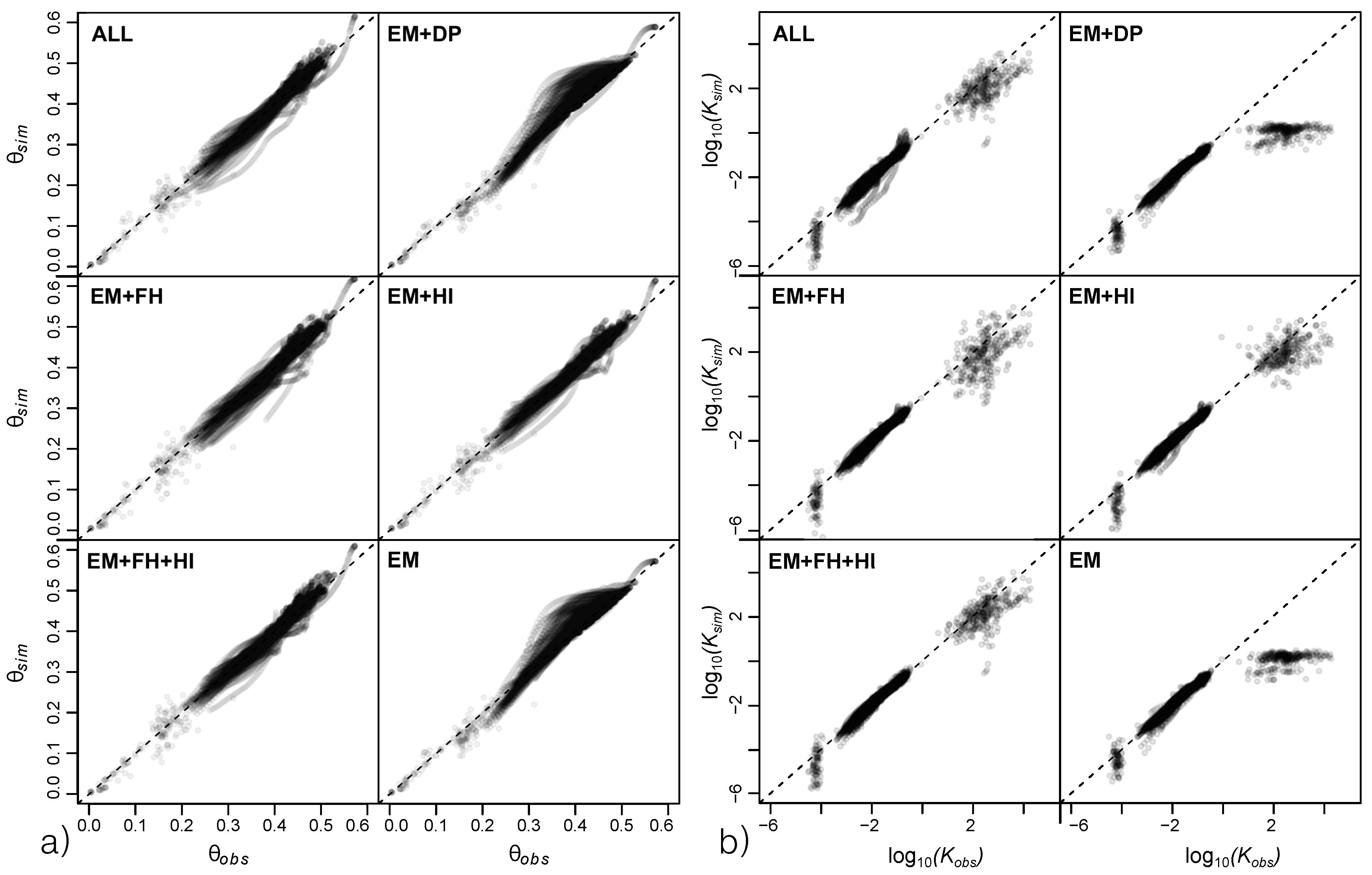
For the water retention curve, data were derived by two methods: EM and DP. Figure 1 shows smooth transition between these methods which was observed for all samples. This was also reported by Schelle et al. [56]. Higher discrepancy occurred in the conductivity curve. Three methods surveyed unsaturated and saturated conductivity: FH, HI, EM. The backbone of the applied measurement procedure was EM as it yielded data for retention and conductivity curve. Nevertheless, by EM only matric flow was observed as no gravity-driven macropore flow occurred in the bottom-sealed experiment. 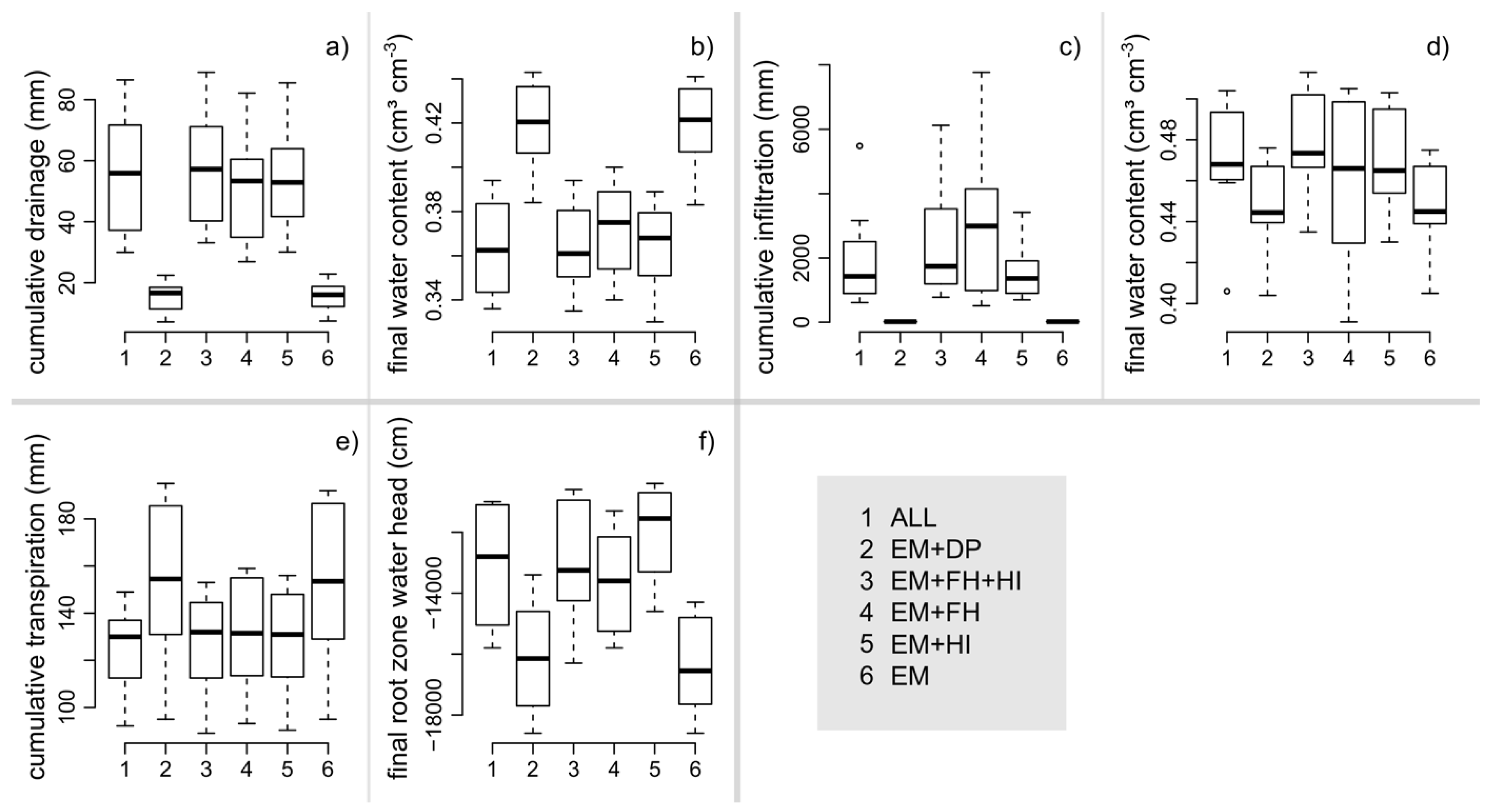In contrast, macropore flow was the dominant flow process in FH and HI experiments and measured values were two to four orders of magnitude higher then maximum conductivity values of EM (Figure 1). Applying a functional approach [31], we could also quantify the effects of these differences. Especially the results for experimental field capacity, infiltration rates, and actual transpiration in a dry period were remarkable and caused by the better representation of macro-pore system with YesCon methods. In contrast, drying simulations did not include drier conditions than h = −15,000 cm. The importance of DP-measurements was supposed to rise during more intensive drying.

The herein applied evaluation procedure was designed on a basic level to keep the focus on the comparison of measurement methods and their combination. Hence, phenomena like hysteresis or shrinking were neglected and arise potential for further research. The sampled soils were silt-dominated, hydrophilic and affected by agricultural management. Consequently, the results are not representative for clay or sand soils, water repellent soils and differing land use systems like forests or fallows.

In a considerable number of fits, the parameters reached their predefined constraints. In concrete studies, this behaviour should be examined in more detail. Especially $\tau$ was highly variable together with high correlation to simulation results. This emphasized a need for further investigation, especially considering the habit to set this parameter to a fixed value in fitting applications (e.g., [57]). Accordingly, Dettmann et al. [58] yielded improved HSP-fits with $\tau$ as free fitting parameter and suggested further modifications of fitting procedures. Additionally, it was surprising that $w_2$, the weighing parameter accounting for bimodality, did not differ between method combinations. Bimodality was expected to be better observable with YesCon but the result might lead to the interpretation that the retention curve includes enough information for determination of bimodality. Nevertheless, the lower variability for $w_2$ in YesCon measurements pointed out more accurate determination of bimodality.

All measurements implied physical impacts on soil structure which might have caused bias in observations of hydraulic soil properties or soil structure. During infiltration measurements in the field, only a small part at the surface of the treated soil volume was exposed to considerable forces. In contrast, undisturbed samples for lab measurements (FH and EM) underwent multiple steps of sample handling also in saturated state where structural stability is lowest. Moreover, the variability of replicated FH measurements was considerably higher than that of HI. This was most likely a result of different sampling volumes—the cross-sectional area of the flow domain for HI (483 cm² at soil surface) was more than nine times larger than that of FH (55 cm²)—and the higher number of measured data pairs (1 for FH, 2–3 for HI). In the small cores, the probability for a continuous macro-pore to control saturated hydraulic conductivity was high, which partly explained the higher variability in FH-measurements.

5. Conclusions

The intention of this study was to quali- and quantitatively evaluate different combinations of measurement methods for the parametrization of hydraulic soil properties functions. Analysing the results and practical considerations, we emphasized the importance of measurements of hydraulic conductivity near saturation as the basis for soil water modelling in silt-dominated, structured, arable soils. We suggested applying infiltration experiments in the field—in our case using hood infiltrometer—additionally to the evaporation method. Compared to lab measurement with falling head method, higher sampling volume and lower error-proneness increased representativeness of parametrization, at least at profile scale. Nevertheless, we still saw a need to extend the measurement range of infiltration experiments to account also for the transition range between macro- and mesopore flow at h = −2.5 to −6.0 cm. Additionally, further research should concentrate on the evaluation of combined measurement procedures for a wider range of land use and soil management systems.

References

1. Assouline, S.; Or, D. Conceptual and Parametric Representation of Soil Hydraulic Properties: A Review. Vadose Zone J. 2013, 12, 108–112. [Google Scholar] [CrossRef]
2. Vereecken, H.; Schnepf, A.; Hopmans, J.; Javaux, M.; Or, D.; Roose, T.; Vanderborght, J.; Young, M.; Amelung, W.; Aitkenhead, M.; et al. Modeling Soil Processes: Review, Key challenges and New Perspectives. Vadose Zone J. 2016, 15, 1–57. [Google Scholar] [CrossRef] [Green Version]
3. Kutilek, M. Soil hydraulic properties as related to soil structure. Soil Tillage Res. 2004, 79, 175–184. [Google Scholar] [CrossRef]
4. Wösten, J.H.M.; Pachepsky, Y.A.; Rawls, W.J. Pedotransfer functions: Bridging the gap between available basic soil data and missing soil hydraulic characteristics. J. Hydrol. 2001, 251, 123–150. [Google Scholar] [CrossRef]
5. Vereecken, H.; Weynants, M.; Javaux, M.; Pachepsky, Y.; Schaap, M.G.; van Genuchten, M. Using Pedotransfer Functions to Estimate the van Genuchten–Mualem Soil Hydraulic Properties: A Review. Vadose Zone J. 2010, 9, 795–820. [Google Scholar] [CrossRef]
6. Dane, J.H.; Topp, G.C.; Campbell, G.S.; Al-Amoodi, L.; Dick, W.A. Methods of Soil Analysis: Physical Methods; Soil Science Society of America: Madison, WI, USA, 2002; p. 1692. [Google Scholar]
7. Gribb, M.M.; Kodesova, R.; Ordway, S.E. Comparison of Soil Hydraulic Property Measurement Methods. J. Geotech. Geoenviron. Eng. 2004, 130, 1084–1095. [Google Scholar] [CrossRef]
8. Nasta, P.; Assouline, S.; Gates, J.B.; Hopmans, J.W.; Romano, N. Prediction of Unsaturated Relative Hydraulic Conductivity from Kosugi’s Water Retention Function. Procedia Environ. Sci. 2013, 19, 609–617. [Google Scholar] [CrossRef]
9. Gribb, M.M.; Forkutsa, I.; Hansen, A.; Chandler, D.G.; McNamara, J.P. The Effect of Various Soil Hydraulic Property Estimates on Soil Moisture Simulations. Vadose Zone J. 2009, 8, 321–331. [Google Scholar] [CrossRef]
10. Nimmo, J.R.; Rubin, J.; Hammermeister, D.P. Unsaturated flow in a centrifugal field: Measurement of hydraulic conductivity and testing of Darcy’s Law. Water Resour. Res. 1987, 23, 124–134. [Google Scholar] [CrossRef]
11. Malengier, B.; Di Emidio, G.; Peiffer, H.; Ciocci, M.C.; Kišon, P. Unsaturated permeability and retention curve determination from in-flight weight measurements in a bench-scale centrifuge. Geotech. Test. J. 2015, 38, 243–254. [Google Scholar] [CrossRef]
12. Fu, X.; Shao, M.; Lu, D.; Wang, H. Soil water characteristic curve measurement without bulk density changes and its implications in the estimation of soil hydraulic properties. Geoderma 2011, 167–168, 1–8. [Google Scholar] [CrossRef]
13. Wind, G. Capillary conductivity data estimated by a simple method. In Proceedings of the UNESCO/IASH Symposion ‘Water in the Unsaturated Zone’, Wageningen, The Netherlands, June 1966; pp. 181–191. [Google Scholar]
14. Schindler, U.; Durner, W.; von Unold, G.; Mueller, L.; Wieland, R. The evaporation method: Extending the measurement range of soil hydraulic properties using the air-entry pressure of the ceramic cup. J. Plant Nutr. Soil Sci. 2010, 173, 563–572. [Google Scholar] [CrossRef]
15. Vachaud, G.; Dane, J.H. Instantaneous Profile. In Methods of Soil Analysis. Part 4—Physical Methods; Soil Science Society of America: Madison, WI, USA, 2002; pp. 937–945. [Google Scholar]
16. Mubarak, I.; Mailhol, J.C.; Angulo-Jaramillo, R.; Ruelle, P.; Boivin, P.; Khaledian, M. Temporal variability in soil hydraulic properties under drip irrigation. Geoderma 2009, 150, 158–165. [Google Scholar] [CrossRef]
17. Hardie, M.A.; Lisson, S.; Doyle, R.B.; Cotching, W.E. Evaluation of rapid approaches for determining the soil water retention function and saturated hydraulic conductivity in a hydrologically complex soil. Soil Tillage Res. 2013, 130, 99–108. [Google Scholar] [CrossRef]
18. Van Dam, J.C.; Stricker, J.N.M.; Droogers, P. Inverse Method to Determine Soil Hydraulic Functions from Multistep Outflow Experiments. Soil Sci. Soc. Am. J. 1994, 58, 647–652. [Google Scholar] [CrossRef]
19. Durner, W.; Iden, S.C. Extended multistep outflow method for the accurate determination of soil hydraulic properties near water saturation. Water Resour. Res. 2011, 47, 427–438. [Google Scholar] [CrossRef]
20. Minasny, B.; Field, D.J. Estimating soil hydraulic properties and their uncertainty: The use of stochastic simulation in the inverse modelling of the evaporation method. Geoderma 2005, 126, 277–290. [Google Scholar] [CrossRef]
21. Angulo-Jaramillo, R.; Vandervaere, J.P.; Roulier, S.; Thony, J.L.; Gaudet, J.P.; Vauclin, M. Field measurement of soil surface hydraulic properties by disc and ring infiltrometers. Soil Tillage Res. 2000, 55, 1–29. [Google Scholar] [CrossRef]
22. Latorre, B.; Peña, C.; Lassabatere, L.; Angulo-Jaramillo, R.; Moret-Fernández, D. Estimate of soil hydraulic properties from disc infiltrometer three-dimensional infiltration curve: Numerical analysis and field application. J. Hydrol. 2015, 527, 1–12. [Google Scholar] [CrossRef]
23. Richard, G.; Sillon, J.; Marloie, O. Comparison of Inverse and Direct Evaporation Methods for Estimating Soil Hydraulic Properties under Different Tillage Practices. Soil Sci. Soc. Am. J. 2001, 65, 215–224. [Google Scholar] [CrossRef]
24. Zhang, K.; Burns, I.G.; Greenwood, D.J.; Hammond, J.P.; White, P.J. Developing a reliable strategy to infer the effective soil hydraulic properties from field evaporation experiments for agro-hydrological models. Agric. Water Manag. 2010, 97, 399–409. [Google Scholar] [CrossRef] [Green Version]
25. Kumahor, S.K.; De Rooij, G.H.; Schlüter, S.; Vogel, H.J. Water Flow and Solute Transport in Unsaturated Sand—A Comprehensive Experimental Approach The investigation of solute transport during unsaturated water flow in soil. Vadose Zone J. 2015, 1, 14. [Google Scholar] [CrossRef]
26. Zhuang, L.; Bezerra Coelho, C.; Hassanizadeh, S.; van Genuchten, M. Analysis of the Hysteretic Hydraulic Properties of Unsaturated Soil. Vadose Zone J. 2017, 16, 1–9. [Google Scholar] [CrossRef]
27. Peters, A.; Durner, W. Simplified evaporation method for determining soil hydraulic properties. J. Hydrol. 2008, 356, 147–162. [Google Scholar] [CrossRef]
28. Mermoud, A.; Xu, D. Comparative analysis of three methods to generate soil hydraulic functions. Soil Tillage Res. 2006, 87, 89–100. [Google Scholar] [CrossRef]
29. Siltecho, S.; Hammecker, C.; Sriboonlue, V.; Clermont-Dauphin, C.; Trelo-Ges, V.; Antonino, A.C.D.; Angulo-Jaramillo, R. Use of field and laboratory methods for estimating unsaturated hydraulic properties under different land uses. Hydrol. Earth Syst. Sci. 2015, 19, 1193–1207. [Google Scholar] [CrossRef]
30. Bennett, N.D.; Croke, B.F.; Guariso, G.; Guillaume, J.H.; Hamilton, S.H.; Jakeman, A.J.; Marsili-Libelli, S.; Newham, L.T.; Norton, J.P.; Perrin, C.; et al. Characterising performance of environmental models. Environ. Model. Softw. 2013, 40, 1–20. [Google Scholar] [CrossRef]
31. Romano, N.; Nasta, P. How effective is bimodal soil hydraulic characterization? Functional evaluations for predictions of soil water balance. Eur. J. Soil Sci. 2016, 67, 523–535. [Google Scholar] [CrossRef]
32. Madi, R.; Huibert De Rooij, G.; Mielenz, H.; Mai, J. Parametric soil water retention models: A critical evaluation of expressions for the full moisture range. Hydrol. Earth Syst. Sci. 2018, 22, 1193–1219. [Google Scholar] [CrossRef]
33. Stumpp, C.; Engelhardt, S.; Hofmann, M.; Huwe, B. Evaluation of pedotransfer functions for estimating soil hydraulic properties of prevalent soils in a catchment of the Bavarian Alps. Eur. J. For. Res. 2009, 128, 609–620. [Google Scholar] [CrossRef]
34. Campbell, E.C.; Campbell, G.S.; Barlow, W.K. A dewpoint hygrometer for water potential measurement. Agric. Meteorol. 1973, 12, 113–121. [Google Scholar] [CrossRef]
35. Klute, A.; Dirksen, C. Hydraulic conductivity and diffusivity: Laboratory methods. In Methods of Soil Analysis. Part 1. Physical and Mineralogical Methods, 2nd ed.; Klute, A., Ed.; American Society of Agronomy: Madison, WI, USA, 1986; pp. 687–734. [Google Scholar]
36. Schwärzel, K.; Punzel, J. Hood Infiltrometer—A New Type of Tension Infiltrometer. Soil Sci. Soc. Am. J. 2007, 71, 1438–1447. [Google Scholar] [CrossRef]
37. Priesack, E.; Durner, W. Closed-Form Expression for the Multi-Modal Unsaturated Conductivity Function. Vadose Zone J. 2006, 5, 121–124. [Google Scholar] [CrossRef]
38. Van Genuchten, M.T. A Closed-form Equation for Predicting the Hydraulic Conductivity of Unsaturated Soils. Soil Sci. Soc. Am. J. 1980, 44, 892. [Google Scholar] [CrossRef]
39. Mualem, Y. A new model for predicting the hydraulic conductivity of unsaturated porous media. Water Resour. Res. 1976, 12, 513–522. [Google Scholar] [CrossRef]
40. Kemper, W.D.; Koch, E.J. Aggregate Stability of Soils from Western United States and Canada. Measurement Procedure, Correlation With Soil Constituents; United State Department of Agriculture: Washington, DC, USA, 1966; pp. 1–57.
41. ÖNORM EN ISO 14688-1:2018-06-15. Geotechnical Investigation and Testing‚ Identification and Classification of Soil‚ Part 1: Identification and Description; Austrian Standards: Vienna, Austria, 2018; p. 22. [Google Scholar]
42. Bagarello, V.; Castellini, M.; Iovino, M. Influence of the Pressure Head Sequence on the Soil Hydraulic Conductivity Determined With Tension Infiltrometer. Appl. Eng. Agric. 2005, 21, 383–391. [Google Scholar] [CrossRef]
43. Matula, S.; Miháliková, M.; Lufinková, J.; Báťková, K. The role of the initial soil water content in the determination of unsaturated soil hydraulic conductivity using a tension infiltrometer. Plant Soil Environ. 2016, 61, 515–521. [Google Scholar] [CrossRef] [Green Version]
44. ÖNORM L 1065:2006-12-01. Physikalische Bodenuntersuchungen—Bestimmung der hydraulischen Leitfähigkeit in gesättigten Zylinderproben; Austrian Standards: Vienna, Austria, 2006. [Google Scholar]
45. METER Group Inc. WP4C Dew Point PotentiaMeter, version ju ed.; METER Group Inc.: Pullman, WA, USA, 2017. [Google Scholar]
46. Simunek, J.; Sejna, M.; Saito, H.; Sakai, M.; van Genuchten, M. The HYDRUS-1D Software Package for Simulating the One-Dimensional Movement of Water, Heat, and Multiple Solutes in Variably-Saturated Media, version 4.08; HYDRUS Software Series 3; Department of Environmental Science, University of California: Riverside, CA, USA, 2009; p. 332. [Google Scholar]
47. Karaboga, D. An Idea Based on Honey Bee Swarm for Numerical Optimization; Technical Report TR06; Erciyes University: Melikgazi/Kayseri, Turkey, 2005; p. 10. [Google Scholar]
48. Vega Yon, G.; Munoz, E. ABCoptim: An Implementation of the Artificial Bee Colony (ABC) Algorithm. Technical Report. 2017. Available online: https://cran.r-project.org/web/packages/ABCoptim/ABCoptim.pdf (accessed on 2 August 2018).
49. Peters, A.; Durner, W. SHYPFIT 2.0 User’s Manual; Technical Report June; Institut für Ökologie, Technische Universität Berlin: Berlin, Germany, 2015. [Google Scholar]
50. Bezerra-Coelho, C.R.; Zhuang, L.; Barbosa, M.C.; Soto, M.A.; Genuchten, M.T.V. Further tests of the HYPROP evaporation method for estimating the unsaturated soil hydraulic properties. J. Hydrol. Hydromech. 2017, 66, 161–169. [Google Scholar] [CrossRef]
51. Feddes, R.; Kowalik, P.; Zaradny, H. Simulation of Field Water Use and Crop Yield; Pudoc: Wageningen, The Netherlands, 1978. [Google Scholar]
52. R Core Team. R: A Language and Environment for Statistical Computing; R Foundation for Statistical Computing: Vienna, Austria, 2016. [Google Scholar]
53. Tukey, J.W. Comparing Individual Means in the Analysis of Variance. Biometrics 1949, 5, 99. [Google Scholar] [CrossRef] [PubMed]
54. De Mendiburu, F. Agricolae: Statistical Procedures for Agricultural Research. R Package Version 1.2-4. 2016. Available online: https://lair.ownr.io/ui/cran/p/agricolae/src (accessed on 2 August 2018).
55. Soil Science Society of America. Glossary of Soil Science Terms; SSSA: Madison, WI, USA, 2008. [Google Scholar]
56. Schelle, H.; Heise, L.; Jänicke, K.; Durner, W. Water retention characteristics of soils over the whole moisture range: A comparison of laboratory methods. Eur. J. Soil Sci. 2013, 64, 814–821. [Google Scholar] [CrossRef]
57. Werisch, S.; Grundmann, J.; Al-Dhuhli, H.; Algharibi, E.; Lennartz, F. Multiobjective parameter estimation of hydraulic properties for a sandy soil in Oman. Environ. Earth Sci. 2014, 72, 4935–4956. [Google Scholar] [CrossRef]
58. Dettmann, U.; Bechtold, M.; Frahm, E.; Tiemeyer, B. On the applicability of unimodal and bimodal van Genuchten-Mualem based models to peat and other organic soils under evaporation conditions. J. Hydrol. 2014, 515, 103–115. [Google Scholar] [CrossRef]
Figure 1. Example of measurements for hydraulic soil properties to illustrate ranges of different methods; 11 replicates measured in one treatment (site B, T1). Subplot (a) is the water retention curve θ ( h ) , (b) is the hydraulic conductivity curve K ( h ) . For both, h is transformed to pF by pF = log 10 | h | .
Water 10 01021 g001
Figure 2. (a) comparison of volumetric water content θ ( h ) (cm3 cm−3) observed ( θ o b s ) and calculated ( θ s i m ) with fitted parameters; (b) comparison of hydraulic soil conductivity K ( h ) (log10 (m day−1)) observed ( K o b s ) and calculated ( K s i m ) with fitted parameters; points are printed in semi-transparent black colour, hence dark parts show high point density; 88 samples included in each subplot.
Water 10 01021 g002
Figure 3. Modelling results. (a) cumulative drainage in mm; (b) final water volume in mm, both from drainage experiment; (c) cumulative infiltration in mm; (d) final water volume in mm, both from infiltration experiment; site-based simulations: (e) transpiration in mm day−1; (f) mean water head in the root zone in cm. Values of (b,d) refer to a soil column of 200 cm depth. Formal statistical analysis is not validly applicable as site and tillage treatment are present in the results as disturbance factors—graph only for visual expression.
Water 10 01021 g003
Figure 4. Development of water head in the root zone (a) and transpiration rate (b) during drying period. Daily values, diurnal variations neglected.
Water 10 01021 g004