Inherent Relationship between Flow Duration Curves at Different Time Scales: A Perspective on Monthly Flow Data Utilization in Daily Flow Duration Curve Estimation

Abstract

Modelling flow duration curves (FDCs) has long been a topic of interest since it is widely used in various hydrological applications. Most studies related to the estimation of FDCs in ungauged or partial gauged basins focus primarily on using climate and catchment characteristics to regionalize FDC at some single time scale. However, the relationship of FDCs at various time scales are rarely analyzed or studied. Here, we propose two methods, which are Modelled FDC Parameter comparison (M-FDC-P) and Empirical FDC Ratio comparison (E-FDC-R), to study the quantitative relationship between daily and monthly FDCs. One method M-FDC-P, selects a Kappa (KAP) distribution to represent the characteristics of the FDCs and then analyzes the relationship between KAP parameters of modelled FDCs at different time scales. Results indicate that three out of four parameters have strong correlations between FDCs at daily and monthly time scales. The other method, E-FDC-R, compares the quantitative relationship between daily and monthly empirical FDCs with given exceedance probabilities. The Power function is used for fitting the ratio-exceedance probability curves. In addition, the simulated daily FDC derived from monthly FDC can be very consistent with the observed daily flow records when the two parameters of power function are quantified precisely. These results clearly indicate that there are strong connections between daily and monthly FDCs, and monthly FDC can provide valuable information for daily FDC estimation. Since flow records at a large time scale are easier to obtain, daily FDC could be derived from monthly FDC by considering the inherent relationships between FDCs at different time scales, which is not sufficiently realized in previous studies.

1. Introduction

The flow duration curve (FDC), which illustrates the percentage of time with which daily, monthly or some other time interval flows are equaled or exceeded over a historical period for a particular river basin, is recognized as one of the most important and widely used signatures of catchment runoff response [1]. The FDC is often interpreted as the complement of the cumulative distribution function of the flow, which provides a graphical representation of the relationship between the frequency and magnitude of flows, making it a compact signature of a catchment’s functioning [2,3].

However, the modeling of FDCs has proven elusive, because of the complicated dynamics existing in flows, such as fractal and multifractal behavior [4], chaos-like dynamics [5,6,7], and periodicity in the mean, standard deviation, and skewness [8]. For example, at the daily time scale, daily flow is a complex time series with flow values ranging over many orders of magnitude [9]. It is very difficult to characterize the probability distribution that can approximate daily flow precisely.

At present, major studies related to the estimation of FDCs in ungauged or partial gauged basins focus primarily on statistical methods, which can be divided into three types [10,11]. The first one is the regression method, which involves establishing the relationship between flow with exceedance probabilities (or flow durations) and a set of climate and catchment characteristics [12,13,14,15]. The second one is the index method, which includes regionalization of parameters that represent the distribution function of FDC [16,17,18]. When no streamflow records are available, regional FDCs are used to synthesize FDCs [19]. The third one is the geostatistical method, which involves relying on kriging methods to produce predictions of hydrologic phenomena at ungauged sites with the combination of the information collected at neighboring gauging stations [20]. Over the past decade, geostatistical approaches predicting streamflow indices in ungauged basins have become increasingly popular [21,22,23,24].

However, as it can be seen, the above researches related with FDC mainly focus on a certain time scale, such as daily or annual. Except very few studies, the existing literature rarely concerns or analyzes the relationships among the FDCs at different time scales. Since FDCs at daily or monthly or annual time scale have different usages in the hydrology [9,25], and flow records at large time scale are easier to obtain, we are curious about the relationship between FDCs at different time scales. Are there any connections among the FDCs at different time scales? Is the information in FDC at large time scale implicit in small time scale? Can large scale FDCs provide some reference for small scale FDC?

To answer these questions, this paper comprehensively studies the correlations between FDCs at different time scales, especially for daily and monthly FDCs. The expected research results will be very important and useful for ungauged or partial gauged basins, which often just have flow records at larger time scale. To achieve this objective, the paper is structured as follows: Section 2 proposes the methodology to calculate the correlations between FDCs at different time scales. Section 3 describes the study area and data used. In Section 4, the variation characteristics of FDCs at different time scales and the correlations between different FDCs are revealed. Section 5 provides a detailed discussion of the results. The last section summarizes the conclusions of this study.

2. Methodology

In the present study, the correlations between FDCs at different time scales are studied by applying two types of methods. One method, called the Modelled FDC Parameter comparison (abbreviated as M-FDC-P), is to calculate the correlations between the parameters of modelled FDCs at different time scales. The other one, called the Empirical FDC Ratio comparison (abbreviated as E-FDC-R), is to compare the ratio relationship of different empirical FDCs with given exceedance probabilities.

2.1. M-FDC-P Method

M-FDC-P method first selects a specific probability distribution for modelling FDCs at different time scales and then compares the correlations between the probability distribution parameters of FDCs. By doing so, it is vivid to see to what degree the parameters are correlated, and which parameter is obviously strongly or weakly correlated.

Previous studies have noted that a complex distribution with at least four parameters is needed to approximate the probability distribution of the daily streamflow [2,16]. Blum et al. [9] demonstrated that four-parameter Kappa (KAP) distribution outperformed other three-parameter distributions and could provide a very good fit to the distribution of daily streamflow across most of the US. KAP distribution [18,25,26] is, therefore, selected as a probability distribution for modelling FDCs at different time scales, and its function is defined as follows:

$$F\left(x\right)={\left\{1-h\left[1-\frac{k}{\alpha }{\left(x-\xi \right)}^{1/k}\right]\right\}}^{1/h}$$

(1)

where ξ is a location parameter, α is a scale parameter, and $k$ and $h$ are shape parameters. The corresponding quantile function is described as:

$$x\left(F\right)=\xi +\frac{\alpha }{k}{\left\{1-(\frac{1-F^h}{h})\right\}}^{1/h}$$

(2)

KAP distribution is a base function of many commonly used three-parameter probability distributions. When k ≠ 0, the general Pareto, generalized extreme value and generalized logistic distributions are all special cases of KAP distribution for h = 1, h = 0 and h = –1, respectively.

KAP distribution parameters are usually estimated by the method of L-moments, in which the first p (number of the unknown parameters in the distribution, 4 for KAP distribution) sample L-moments or L-ratios is equaled to the corresponding population quantities. Estimates of L-moment ratios exhibit substantially less bias than ordinary moment ratio estimators and are resistant to the influence of data outliers [26]. Vogel and Fennessey [1], Hosking and Wallis [26] among others have described and summarized the advantages of L-moments, and therefore they are not reproduced herein. The detail description of the theory of L-moments and parameter estimation of KAP distribution can be found in [27,28].

When the probability distribution function is chosen, parameter is the only factor that affects the variation of the probability distribution. Finally, the correlation among KAP distribution parameters at different time scales are evaluated by the most widely used linear correlation coefficient to analyze the relationship between FDCs at different time scales.

2.2. E-FDC-R Method

The above M-FDC-P method uses theoretical probability distribution to model FDCs and then compares the relationship between parameters at different time scales, which may not be universally applicable due to the subjective choice of the probability distribution function. Therefore, the study also selects another way, called E-FDC-R, which does not consider specifying any probability distribution. The steps of the E-FDC-R method are presented as follows:

• Estimation of the empirical FDCs. An empirical FDC is constructed by ranking flows at specific time scales from all recorded years and plotting them against an estimate of their exceedance probability, known as a plotting position [1]. The first step in empirical FDC construction is to sort flow data from highest to lowest. For the probability with which each flow is exceeded, the Weibull plotting position is then used, as it provides an unbiased estimate of exceedance probability, regardless of the underlying probability distribution of the ranked observations [1]. The Weibull plotting position is described as follows:

  $$p=\frac{m}{N+1}\times 100\%$$

  (3)

  where p is the exceedance probability for the mth flow data, and N is the number of the total flow records. Plot p on x axis and the corresponding flow (the mth flow value) on y axis. The plotted dots and the x and y axis form the empirical FDC.
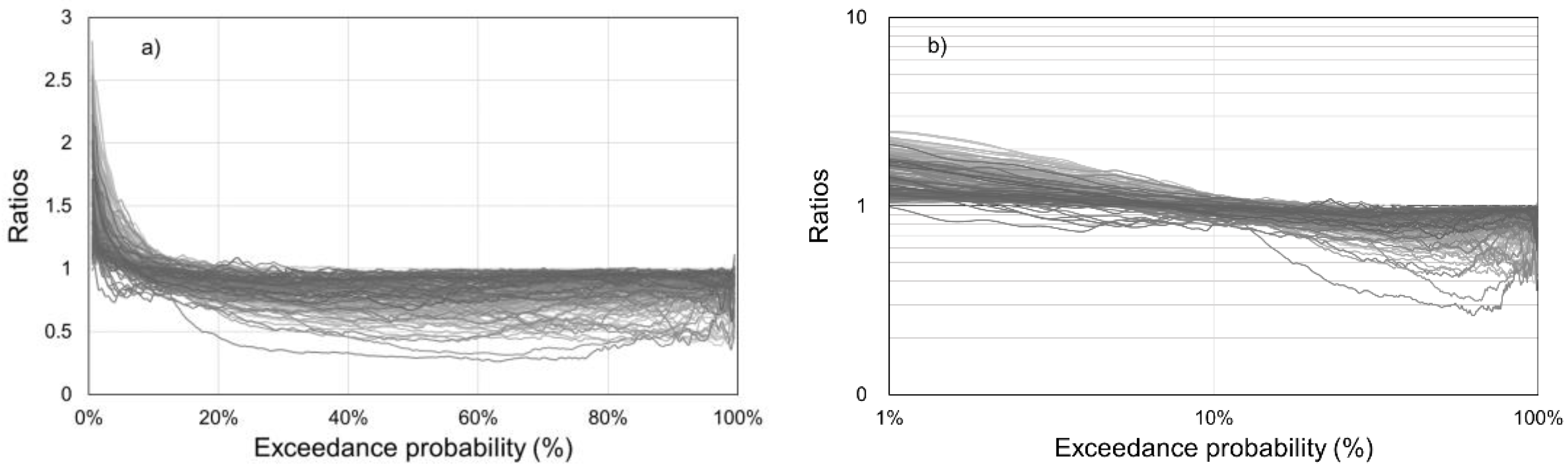
• Calculation of the ratios between empirical FDCs. Firstly, sample a series of flow with pre-selected exceedance probabilities of empirical FDCs at different time scales, and then calculate the ratios of flow values at different time scales with given exceedance probabilities. Thus, the quantitative relationship of FDCs at different time scales is achieved. It should be noted that the number of pre-selected exceedance probabilities needs to be large enough to sufficiently represent the ratio relation of FDCs. Secondly, the quantitative relationship is analyzed in order to find a certain function to represent the quantitative relationship between FDCs.
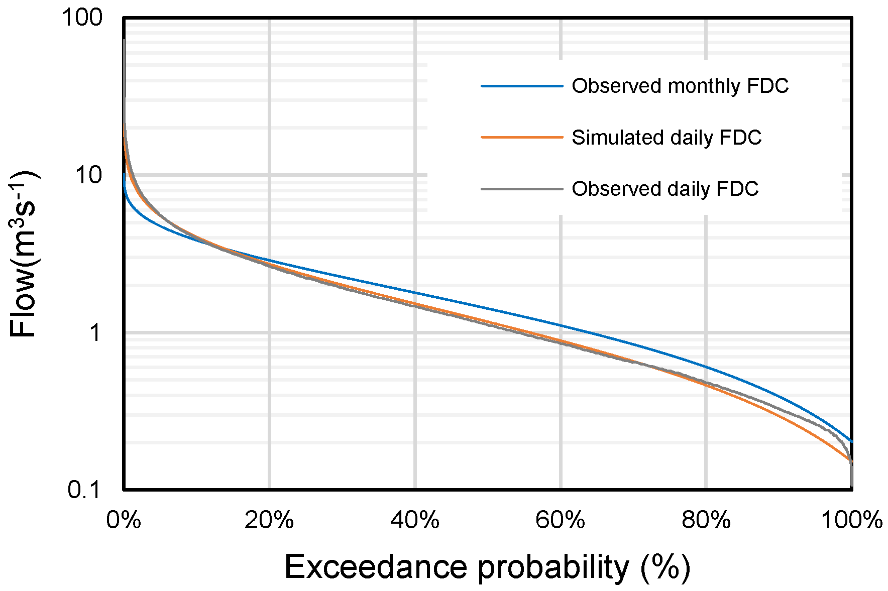
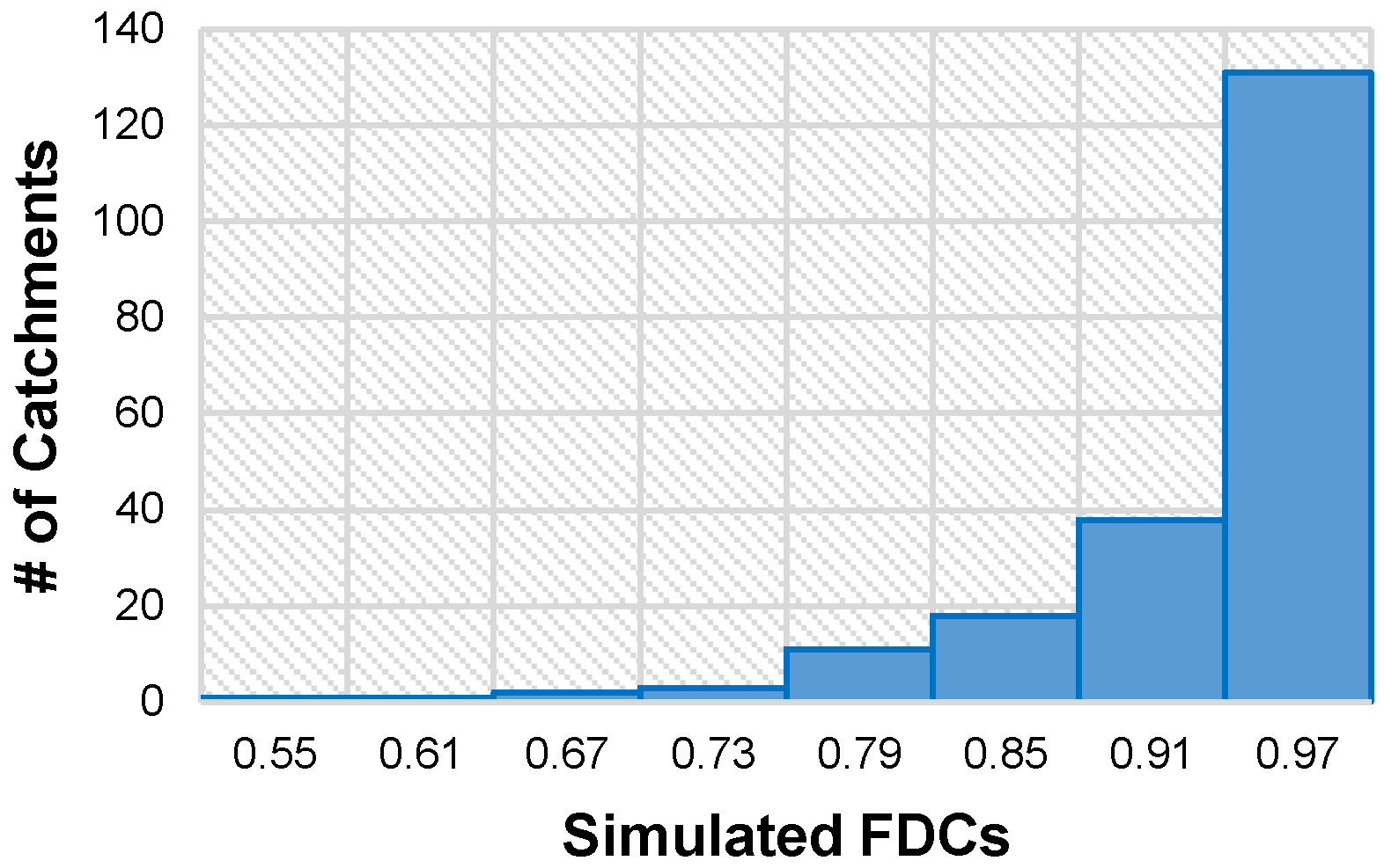
• Evaluation of Modelled FDC. Once the specific function is obtained, the FDC at smaller time scale can be derived via the empirical FDC at larger time scale. To evaluate the performance of FDC at smaller time scale to reproduce observations, a measure of the standardized mean square error commonly referred to as Nash–Sutcliffe efficiency (NSE) is used. The description of NSE is introduced in [9], and hence not reproduced herein.

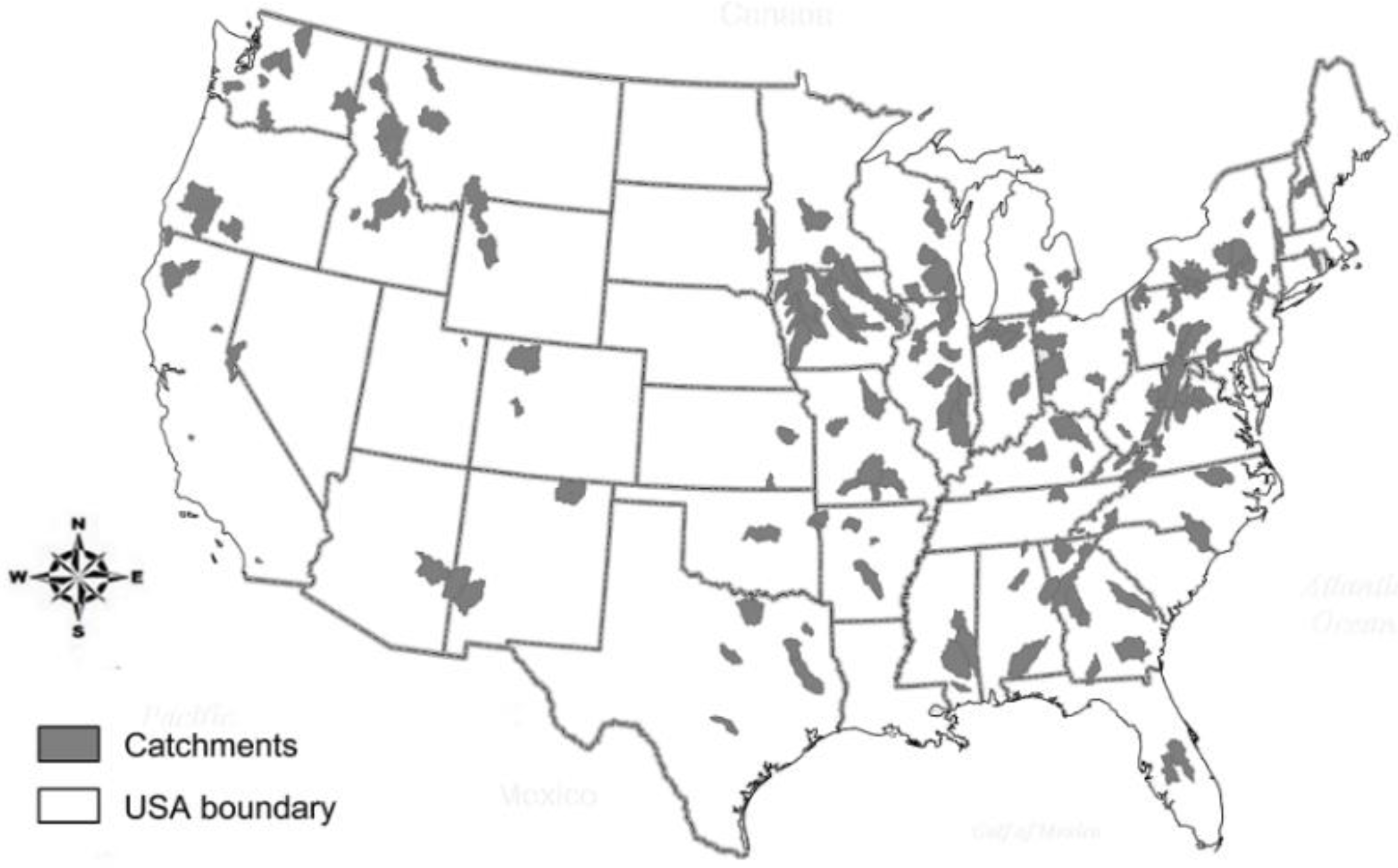
3. Study Area and Data

To keep the accuracy of the research data and the repeatability of the research, the international Model Parameter Estimation Experiment (MOPEX) data set is used in this study. The data set is described by Duan et al. [29] and can be downloaded from ftp://hydrology.nws.noaa.gov/. This data set includes mean areal precipitation, potential evaporation, daily streamflow, and daily maximum and minimum air temperature with an adequate number of precipitation gauges. As this study focuses on FDCs, only the streamflow for 219 catchments in the MOPEX data set is selected for analysis. Most of the streamflow data are included in the Hydroclimatic Data Network (HCDN) [30], which includes only gauges believed to be unaffected by upstream regulations [31] and therefore considered to represent near-natural hydrological conditions, without the need to worry that modifications to streamflow could have substantial impacts on FDCs [10,32]. The MOPEX data set consists of 56 years of daily streamflow from 1948 to 2003, which is long enough to construct FDCs. The catchment locations and boundaries are shown in Figure 1.

4. Results and Analysis

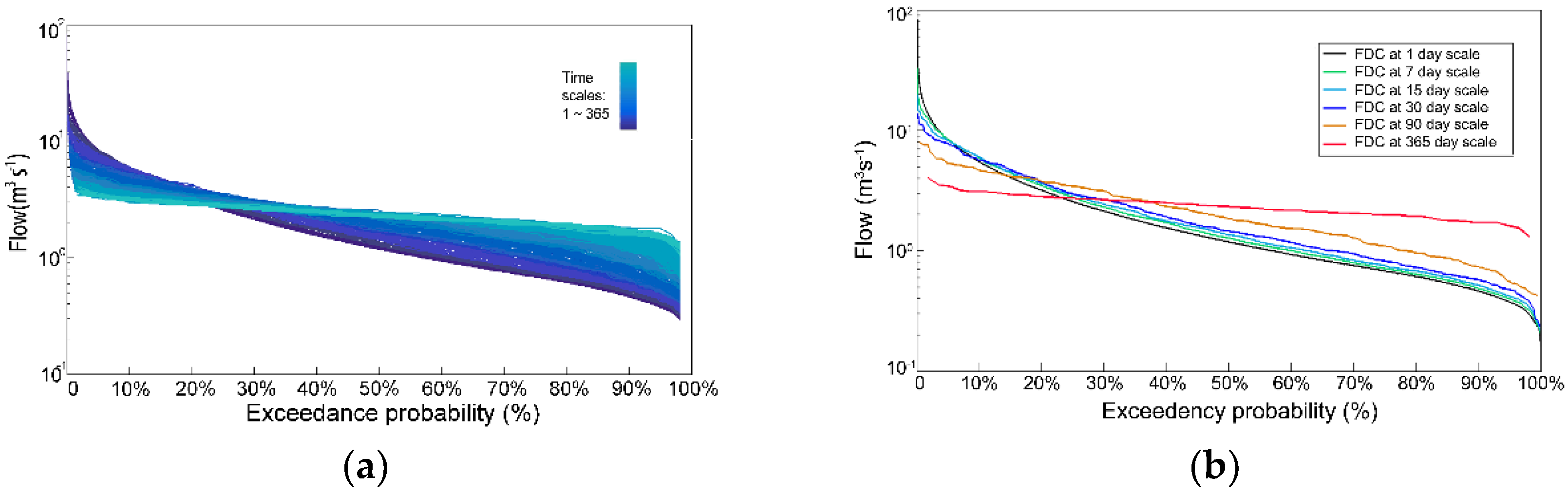
4.1. Empirical FDCs Variation with Different Time Scales

To see how the FDC variations with time scales, Figure 2 displays the empirical FDCs for a randomly selected catchment (No. 1064500) at time scales from 1 day to 365 days. It is evident from Figure 2a that the empirical FDCs change slowly with time scales, which means two FDCs could be very alike when their time scales are not much different, indicating that information of FDC at large time scale might be somewhat implicit in small time scales. FDC at a time scale of 1 day is the steepest (having largest slope) with obvious high flow values for low exceedance probabilities and low flow values for high exceedance probabilities, which then becomes flatter as the time scale gets larger. This is due to the fact that extreme flow events usually occur at the smaller time scale, and larger time scale flow will aggregate the difference, therefore resulting in flat FDC.

Figure 2b shows the empirical FDCs at time scales 1, 7, 15, 30, 90, and 365 days, corresponding to daily, weekly, half-monthly, monthly, seasonally, and yearly FDCs. The empirical FDCs at 1 day to 30 day time scales are very similar. Obvious differences occur when the time scale is larger than 90 days. Therefore, it is logical to investigate the possibilities of estimating daily FDC by using monthly flow data, since monthly flow data is far easier to obtain in the real world.

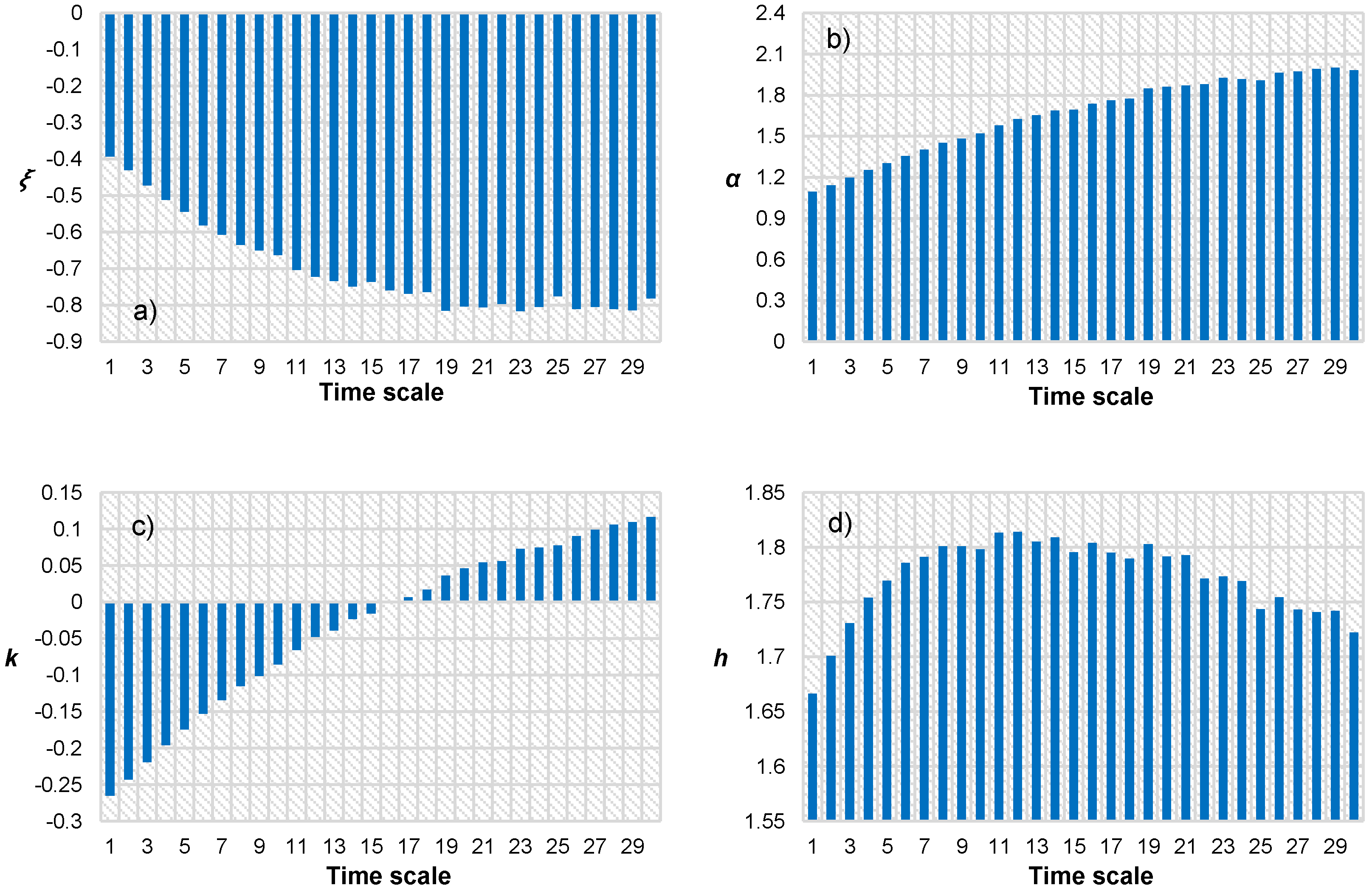
4.2. Relationships of FDCs Derived via M-FDC-P

The daily flow data is averaged at different time scales and then fitted to a KAP distribution, and the relationships of the parameters of the KAP distribution is studied. As demonstrated earlier, the empirical FDCs at 1 to 30 day scales are very similar and might have strong correlations, therefore, this paper concentrates research interest on time scales from 1 to 30 days.

To assess how the KAP distribution parameters vary across time scales, Figure 3 presents the average of four KAP parameters of modelled FDCs for 219 catchments at time scales from 1 to 30 days. It can be seen that all the parameters change gradually with these time scales, some parameters even show a distinct changing trend. The maximum ξ (~−0.4) occurs at a time scale of 1 day and then ξ decreases step by step, and finally stays steady around −0.8 after 19 days. For parameter α, it increases with time scales from 1 day to 30 days, with a minimum 1.1 at 1 day scale and a maximum around 2 at the 29 day scale. k is very similar to α; it increases along with all the time scales from negative to positive, and is very closed to zero at a time scale of 16 days. Parameter h is a little complicated compared to other parameters, for it first increases from 1 day to 11 day time scales and then decreases slightly until 30 day time scales.

The correlations of the four KAP distribution parameters for 219 catchments at different time scales are also studied. The linear correlation coefficients between four parameters at 1, 7, 15, and 30 day time scales are calculated in

Table 1. Linear correlation coefficients between four KAP parameters at different time scales.

Parameter	ξ				α				k				h
Time Scale	1 Day	7 Day	15 Day	30 Day	1 Day	7 Day	15 Day	30 Day	1 Day	7 Day	15 Day	30 Day	1 Day	7 Day	15 Day	30 Day
1 day	1	0.959	0.901	0.858	1	0.953	0.893	0.835	1	0.867	0.654	0.475	1	0.987	0.967	0.940
7 day	0.959	1	0.982	0.954	0.953	1	0.981	0.941	0.867	1	0.931	0.817	0.987	1	0.992	0.973
15 day	0.901	0.982	1	0.990	0.893	0.981	1	0.985	0.654	0.931	1	0.962	0.967	0.992	1	0.992
30 day	0.858	0.954	0.990	1	0.835	0.941	0.985	1	0.475	0.817	0.962	1	0.940	0.973	0.992	1

. For parameter ξ, all the correlation coefficients exceed 0.85, indicating very high correlations exist in parameter ξ at 1 to 30 days. The linear correlation coefficients between 1 day and other days become smaller as the time scale gets larger, so does the other time scales. It can also be seen in Table 1, except that the correlation coefficient for α between the largest time scale difference of 1 day and 30 day is 0.835; all the other correlation coefficients are higher or much closed to 0.9, which also indicates that high correlations exist in parameter α at 1 to 30 day. However, when compared to ξ, the correlations of α at different scales are a little weaker. When looking at parameter k, the linear correlation coefficients are dramatically lower than parameters ξ and α, with lowest correlation coefficients between 1 day and 30 day less than 0.5, indicating very weak correlation. The correlation coefficients for parameter h between 1 day and other days become smaller as the time scale gets larger, just like other parameters. The linear correlation coefficients for h are the highest of all the parameters, with the lowest correlation coefficient between 1 day and 30 day still passing 0.94, indicating an extremely strong correlation.

In addition, the relationships of the four parameters at different times are also studied by plotting corresponding parameter values for all the catchments. For illustration, the four parameters at the largest time scale difference of 1 day and 30 day are plotted in Figure 4. For parameter ξ, most of the points lie in or very near to the regression line. By comparing the linear correlation coefficients and the plot, it is easily to see the degree to which ξ1 can be linear regressed by ξ30. It can also be seen in Figure 4, that although most of the points lie in or very near to the regression line, there are more points far away from the regression line compared to parameter ξ. Meanwhile, these points are very centrally distributed, with a large proportion of points falling in the region bounded by α1 less than 2 and α30 less than 3. When looking at parameter k, the points are much dispersed distributed, and only a few proportion of the points lie in or near to the regression line. Further, these points do not follow a clear relationship, which indicates 𝑘30 is far less informative to estimate 𝑘1 and more information should be incorporated. For parameter h, it can be seen that except few points away from the regression line, most of the points lie in or very near to the regression line, which indicates that simple linear regression can have good performance for estimating h1 when only h30 is available.

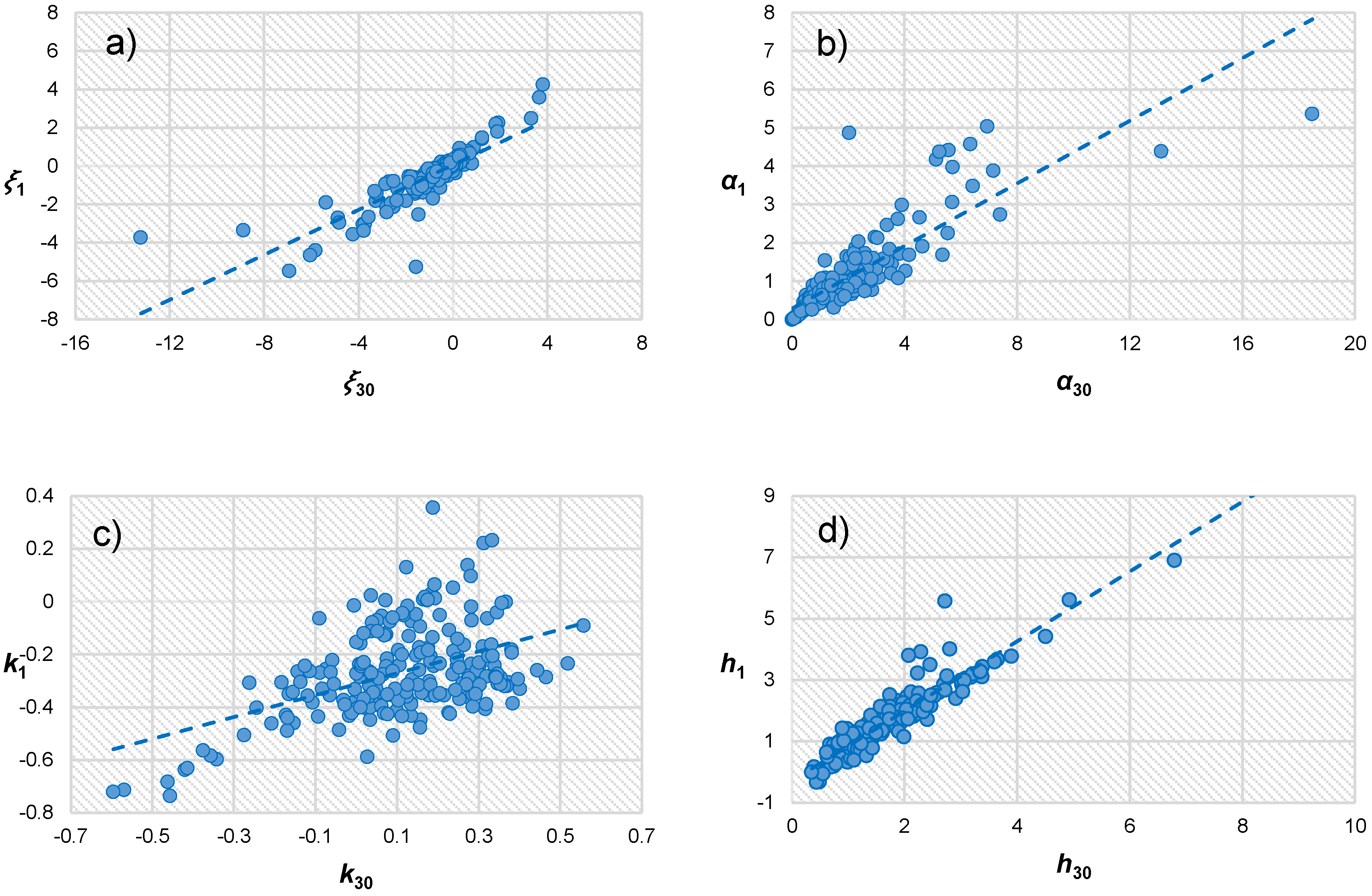
4.3. Relationships of FDCs Derived via E-FDC-R

Here we also focus research interest on the correlation between the FDCs at 1 day and 30 day. The flow values corresponding to 1 day and 30 day are sampled from the exceedance probabilities 0.5% to 99.5% with 0.5% as the sample interval. The total number of the sampled value is 199, which is large enough to analyze the quantitative relationship of FDCs at two time scales.

The ratios of FDC flow values at time scale 1 day to 30 day corresponding to sampled exceedance probabilities are shown in Figure 5. It is evident from Figure 5a that the ratio lines have distinct decreasing trend, these lines firstly decrease dramatically within 20% exceedance probability and slightly decrease thereafter. This is easy to understand that in flood season, maximum daily flow is certainly much higher than the monthly average, so the ratios at low exceedance probabilities are very high. While in non-flood season, minimum daily flow is also far lower than the monthly average, so the ratios at low exceedance probabilities are very low. Consequently, the ratio lines clearly show that daily FDC has higher flow values for low exceedance probability and lower flow values for high exceedance probability compared to monthly FDC, which is also consistent with Figure 2. It should also be noted that most of the curves reach 1 at less than 10% exceedance probability, consistent with [33], in which daily and monthly FDC curves normally cross (representing the ratio equals to 1) between the 1% and 10% exceedance probability in South Africa.

Seen from Figure 5a, the ratio relationship appears to be a power function, we apply the log-log transformation to the ratio relationship. It is evident from Figure 5b that the relationship between ratio value and exceedance probability is overall near-linear in the log-log plot, except a very small proportion in the very high exceedance probability. Here, the power function is used to fit the ratio curves as follows:

$$y=a{x}^{-b}$$

(4)

where x is the exceedance probability; y is the ratio value.

For each catchment, the parameter a and b are estimated and shown in Figure 6. The parameter a for all the catchments is positive and less than 1. This is due to the fact that the ratio is less than 1 for medium and has high exceedance probability. Despite for only two catchments, the parameter b for the rest of the catchments is negative; this is simply because the ratio curve is decreasing overall.

By applying the power function to fit the ratio of daily to monthly FDCs, the daily flow at given exceedance probability can be estimated based on the monthly FDC. The simulated daily FDC for a randomly selected catchment is presented in Figure 7. It is evident that an obvious improvement has been made for simulated daily FDC as it is much closer to daily FDC. Especially for the exceedance probability ranging from 10~70%, the simulated daily FDC and the observed daily FDC almost overlap.

After graphical comparison with observed daily FDC, the simulated daily FDC is modelled by KAP distribution and then evaluated with observed daily flow data. Figure 8 presents the NSE of modelled daily FDC. It is obvious that most of the catchments have very high NSE with median higher than 0.96. The results confirm again that power function is an appropriate relationship for the ratio of daily to monthly FDCs. After power transformation, the modelled daily FDC with good accuracy can be obtained based on monthly FDC.

5. Discussion

The present study aims to ascertain the relationships between FDCs at different time scales, based on M-FDC-P and R-FDC-P. Note that the two methods use different ways to examine the relationships, and some research results are discussed here.

In previous studies, the value of every single parameter of KAP distribution is rarely presented or discussed, though Parida [34] have done some research on the restrictions of the four parameters. In the present research, the averages of four KAP distribution parameters at time scales from 1 to 30 days are analyzed. The relationship between parameter h at 1 and 30 day is so strong that h₁ can be well estimated by merely h₃₀. The high correlation or insensitive of the h parameter is to be expected, as the generalized Pareto, a special case of KAP when h = 1, has been used to describe daily FDCs in many studies [16,18,25]. Even Blum et al. [9] illustrated that there are some regions in the United States such as New England, the Appalachian, and Valley and Ridge regions, for which the generalized Pareto distribution can provide a very good fit to daily FDCs. However, the relationship of the other three parameters are not following a very obvious linear trend or even a single trend (for parameter k). As stated before, even modeling daily FDC in daily gauged sites is very difficult, we are not expecting a single relationship can be found to estimate daily FDC parameters by using only monthly FDC parameters. Therefore, this paper proves that FDC parameters at different time scales are correlated and the relationships found in the paper can be used as an important supplement to the regional regression models to estimate daily FDC at ungauged or partial gauged sites.

As far as the E-FDC-R is concerned, Smakhtin [35] described a method to estimate daily FDCs from monthly flow data, which first assumed that both daily and monthly FDCs are linear in a log-normal space and then established the regression relationship for only two daily FDC indices based on monthly flow data. This method is very ambitious because it established the indices for 200 gauged hydrological stations without any specific parameters representing at-site characteristics. Sugiyama et al. [36] also stated that a distribution of FDC at given exceedance probability was usually represented with a straight line on log-normal probability paper. However, as for the ratio curves of flow values at given exceedance probability, they are very like exponential curves in our work, thus we use the power function to simulate the ratio curves and apply the log-log transformation to the ratio relationship. The results show that the relationship between ratio value and exceedance probability almost tends to be near-linear in the log-log axis, except a very small proportion in the very high exceedance probability. Future studies will consider further improving power function by using a piecewise function to describe the ratio curves for some kind of region (e.g., the stations with positive parameter b after figuring out a way to regionalize parameters in the power function).

6. Conclusions

This study provides a comprehensive assessment of relationships between FDCs at different time scales based on two methods including M-FDC-P and E-FDC-R. Selecting the MOPEX as the research data, the correlations of daily FDC and monthly FDC are deeply analyzed.

As for the M-FDC-P method, the Kappa (KAP) distribution is selected in this work to represent the streamflow distribution characteristics, due to the already existed existing research. The averages of all four KAP parameters tend to change gradually with time scales from 1 to 30 day. Meanwhile, three out of four parameters have linear correlations except the shape parameter k. The relationships found in the paper can be used as an important supplement to the regional regression models to estimate daily FDC at ungauged sites, when observed records with larger time scales are available.

As for the E-FDC-R method, it tries to quantify the relationship between daily and monthly FDCs, based on the ratio of FDCs rather than parameters of a specific distribution. Power function seems to be an effective functions for depicting the relationship between daily and monthly FDCs. The simulated daily FDC derived from monthly FDC can be very consistent with the observed daily flow records, when the two parameters in power function are quantified precisely. There are only two parameters in the power function that need to be regionalized by the site climate and catchment characteristics, which can reduce the uncertainties compared to other regional FDC methods that involve more parameters. Further, the parameter a in power function mainly controls the ratio for high exceedance probability or low flow data; and the parameter b mainly controls the shape of the ratio curve for low exceedance probability or high flow data.

Generally, results based on the above two methods clearly prove that there are strong connections between daily and monthly FDCs, which is not sufficiently realized in previous studies. If a specific probability distribution is applied for modelling FDCs at larger time scales, the gradual change characteristics of the distribution parameters for different FDCs can be considered to provide valuable information for daily FDC estimation. If there is no enough information to ascertain the probability distribution, the simple ratio relationships between different FDCs can help to assess the smaller time scale FDCs. Therefore, the inherent relationship between different FDCs will be very helpful for flow regulation and water resources management, especially in ungauged or partially gauged basins. Nonetheless, our future research will consider the regionalization of the distribution parameters to provide a complete daily FDC estimation using monthly flow data and other information collectively.

References

1. Vogel, R.M.; Fennessey, N.M. L moment diagrams should replace product moment diagrams. Water Resour. Res. 1993, 29, 1745–1752. [Google Scholar] [CrossRef]
2. LeBoutillier, D.W.; Waylen, P.R. A stochastic model of flow duration curves. Water Resour. Res. 1993, 29, 3535–3541. [Google Scholar] [CrossRef]
3. Cheng, L.; Yaeger, M.; Viglione, A.; Coopersmith, E. Exploring the physical controls of regional patterns of flow duration curves—Part 1: Insights from statistical analyses. Hydrol. Earth Syst. Sci. 2012, 9, 4435–4446. [Google Scholar] [CrossRef] [Green Version]
4. Zhang, Q.; Xu, C.Y.; Chen, Y.D.; Yu, Z. Multifractal detrended fluctuation analysis of streamflow series of the Yangtze River basin, China. Hydrol. Process. 2008, 22, 4997–5003. [Google Scholar] [CrossRef]
5. Sivakumar, B. Chaos theory in geophysics: Past, present and future. Chaos Soliton Fract. 2004, 19, 441–462. [Google Scholar] [CrossRef]
6. Wang, W.; Vrijling, J.K.; van Gelder, P.H.A.J.M.; Ma, J. Testing for nonlinearity of streamflow processes at different timescales. J. Hydrol. 2006, 322, 247–268. [Google Scholar] [CrossRef]
7. Tung, W.W.; Gao, J.; Hu, J.; Yang, L. Detecting chaos in heavy-noise environments. Phys. Rev. E 2011, 83, 046210. [Google Scholar] [CrossRef] [PubMed]
8. Bowers, M.C.; Tung, W.W.; Gao, J.B. On the distributions of seasonal river flows: Lognormal or power law? Water Resour. Res. 2012, 48, 5536. [Google Scholar] [CrossRef]
9. Blum, A.G.; Archfield, S.A.; Vogel, R.M. On the probability distribution of daily streamflow in the United States. Hydrol. Earth Syst. Sci. 2017, 21, 3093–3103. [Google Scholar] [CrossRef]
10. Castellarin, A.; Botter, G.; Hughes, D.A.; Liu, S.; Ouarda, T.B.M.J.; Parajka, J.; Post, D.A.; Sivapalan, M.; Spence, C.; Viglione, A.; et al. Prediction of flow duration curves ungauged basins. In Runoff Prediction in Ungauged Basins: Synthesis Across Processes, Places and Scales; Blöschl, G., Sivapalan, M., Wagener, T., Viglione, A., Savenije, H., Eds.; Cambridge University Press: Cambridge, UK, 2013; p. 465. [Google Scholar]
11. Hsu, N.S.; Huang, C.J. Estimation of Flow Duration Curve at Ungauged Locations in Taiwan. J. Hydrol. Eng. 2017, 22, 05017009. [Google Scholar] [CrossRef]
12. Chiang, S.M. Hydrologic Regionalization of Watersheds. II: Applications. J. Water Res. Plan. Manag. 2002, 128, 12–20. [Google Scholar] [CrossRef]
13. Mohamoud, Y. Prediction of daily flow duration curves and streamflow for ungauged catchments using regional flow duration curves. Hydrol. Sci. J. 2008, 53, 706–724. [Google Scholar] [CrossRef] [Green Version]
14. Hope, A.; Bart, R. Synthetic monthly flow duration curves for the Cape Floristic Region, South Africa. Water SA 2012, 38, 191–200. [Google Scholar] [CrossRef]
15. Shu, C.; Ouarda, T.B.M.J. Improved methods for daily streamflow estimates at ungauged sites. Water Resour. Res. 2012, 48, 2523. [Google Scholar] [CrossRef]
16. Castellarin, A.; Galeati, G.; Brandimarte, L.; Montanari, A.; Brath, A. Regional flow-duration curves: Reliability for ungauged basins. Adv. Water Resour. 2004, 27, 953–965. [Google Scholar] [CrossRef]
17. Li, M.; Shao, Q.; Zhang, L.; Chiew, F.H.S. A new regionalization approach and its application to predict flow duration curve in ungauged basins. J. Hydrol. 2010, 389, 137–145. [Google Scholar] [CrossRef]
18. Mendicino, G.; Senatore, A. Evaluation of parametric and statistical approaches for the regionalization of flow duration curves in intermittent regimes. J. Hydrol. 2013, 480, 19–32. [Google Scholar] [CrossRef]
19. Yu, P.S.; Yang, T.C.; Liu, C.W. A regional model of low flow for southern Taiwan. Hydrol. Process. 2010, 16, 2017–2034. [Google Scholar] [CrossRef]
20. Pugliese, A.; Farmer, W.H.; Castellarin, A.; Archfield, S.A.; Vogel, R.M. Regional flow duration curves: Geostatistical techniques versus multivariate regression. Adv. Water Resour. 2016, 96, 11–22. [Google Scholar] [CrossRef]
21. Chokmani, K.; Ouarda, T.B.M.J. Physiographical space-based kriging for regional flood frequency estimation at ungauged sites. Water Resour. Res. 2004, 40, 1–13. [Google Scholar] [CrossRef]
22. Skoien, J.O.; Merz, R.; Bloschl, G. Top-kriging-geostatistics on stream networks. Hydrol. Earth Syst. Sci. 2006, 2, 2253–2286. [Google Scholar] [CrossRef]
23. Castiglioni, S.; Castellarin, A.; Montanari, A. Prediction of low-flow indices in ungauged basins through physiographical space-based interpolation. J. Hydrol. 2009, 378, 272–280. [Google Scholar] [CrossRef]
24. Archfield, S.A.; Pugliese, A.; Castellarin, A.; Skøien, J.O. Topological and canonical kriging for design-flood prediction in ungauged catchments: An improvement over a traditional regional regression approach? Hydrol. Earth Syst. Sci. 2013, 9, 1575–1588. [Google Scholar] [CrossRef]
25. Castellarin, A.; Camorani, G.; Brath, A. Predicting annual and long-term flow-duration curves in ungauged basins. Adv. Water Resour. 2007, 30, 937–953. [Google Scholar] [CrossRef]
26. Hosking, J.R.M.; Wallis, J.R. Regional Frequency Analysis: An Approach Based on L-Moments; Cambridge University Press: Cambridge, UK, 1997; p. 244. [Google Scholar]
27. Hosking, J.R.M. L-moments: Analysis and estimation of distributions using linear combinations of order statistics. J. R. Stat. Soc. B Methodol. 1990, 52, 105–124. [Google Scholar]
28. Kjeldsen, T.R.; Ahn, H.; Prosdocimi, I. On the use of a four-parameter kappa distribution in regional frequency analysis. Hydrol. Sci. J. 2017, 62, 1–10. [Google Scholar] [CrossRef]
29. Duan, Q.; Schaakeb, J.; Andréassian, V.; Franks, S.; Gotetie, G.; Gupta, H.V.; Gusev, Y.M.; Habet, F.; Hall, A.; Hay, L.; et al. Model Parameter Estimation Experiment (MOPEX): An overview of science strategy and major results from the second and third workshops. J. Hydrol. 2006, 320, 3–17. [Google Scholar]
30. Slack, J.R.; Lumb, A.M.; Landwehr, J.M. Hydro-climatic data network (HCDN): A U.S. Geological Survey streamflow data set for the United States for the study of climate variation, 1874–1988. J. Phys. Chem. C 1992, 113, 2538–2544. [Google Scholar]
31. Wang, D.; Hejazi, M. Quantifying the relative contribution of the climate and direct human impacts on mean annual streamflow in the contiguous United States. Water Resour. Res. 2011, 47, 411. [Google Scholar] [CrossRef]
32. Kroll, C.N.; Croteau, K.E.; Vogel, R.M. Hypothesis tests for hydrologic alteration. J. Hydrol. 2015, 530, 117–126. [Google Scholar] [CrossRef]
33. Smakhtin, V.Y.; Watkins, D.A. Low Flow Estimation in South Africa; Report No 494/1/97; Water Research Commission: Pretoria, South Africa, 1997. [Google Scholar]
34. Parida, B.P. Modelling of Indian Summer Monsoon Rainfall Using a Four-parameter Kappa Distribution. Int. J. Climatol. 1999, 19, 1389–1398. [Google Scholar] [CrossRef]
35. Smakhtin, V.U. Estimating daily flow duration curves from monthly streamflow data. Water SA 2000, 26, 13–18. [Google Scholar]
36. Sugiyama, H.; Vudhivanich, V.; Whitaker, A.; Lorsirirat, K. Stochastic Flow Duration Curves for Evaluation of Flow Regimes in Rivers. J. Am. Water Resour. Assoc. 2007, 39, 47–58. [Google Scholar] [CrossRef]
Figure 1. Locations and boundaries of 219 MOPEX catchments.
Water 10 01008 g001
Figure 2. Empirical flow duration curve (FDC) variations with time scales for a randomly selected catchment. (a) Time scales from 1 day to 365 days. (b) Time scales at 1, 7, 15, 30, 90, and 365 days.
Water 10 01008 g002
Figure 3. Variations of average four-parameter Kappa (KAP) parameters at time scales from 1 day to 30 day; (a) parameter ξ; (b); parameter α; (c) parameter k; (d) parameter h.
Water 10 01008 g003
Figure 4. Scatter plots of four parameters at time scales 1 day and 30 day; (a) parameter ξ; (b); parameter α; (c) paramter k; (d) parameter h.
Water 10 01008 g004
Figure 5. Ratios of daily to monthly FDCs at given exceedance probabilities; (a) conventional coordinates; (b) double logarithmic coordinates.
Water 10 01008 g005
Figure 6. Histograms of parameters (a,b) in the power function.
Water 10 01008 g006
Figure 7. Simulated daily FDC based on monthly FDC.
Water 10 01008 g007
Figure 8. NSE of simulated daily FDCs based on monthly FDC.
Water 10 01008 g008