Vulnerability Analysis of the Venetian Littoral and Adopted Mitigation Strategy


ICEA Department, Padua University, v. Ognissanti 39, 35129 Padova, Italy
*
Author to whom correspondence should be addressed.
Water 2018, 10(8), 984; https://doi.org/10.3390/w10080984
Submission received: 30 May 2018
/
Revised: 13 July 2018
/
Accepted: 24 July 2018
/
Published: 26 July 2018
(This article belongs to the Special Issue Coastal Vulnerability and Mitigation Strategies: From Monitoring to Applied Research
)
Abstract
:This paper discusses the key aspects of the recent Coastal Plan of the Veneto Region (IT). Its aim is to propose a single mitigation strategy for coastal erosion that is valid for the whole Veneto Region, and possibly elsewhere, as well as a method to assign a priority level to any action. The suggested mitigation action against erosion depends on urbanization level, beach width, as well as cross-shore and long-shore sediment transport. The criterion used to give a priority level to mitigation actions is based on a vulnerability index that takes into account erosive tendency, existing coastal flooding hazards, coast value, environmental relevance, tourist pressure, urbanization level, the presence of production activities, and cultural heritage. A sample case featuring the littoral of Rosolina is also provided and includes a site description, the sediment budget, critical issues and possible mitigation measures.
1. Introduction
In the recent past, in Italy, when coastal managers at the Regional Authorities were faced with coastal erosion problems, they were frequently guided by an empirical approach based on simple transport equations, or even solely by their intuition. More recently, however, the perspective has changed somewhat and it has become evident that the complexity of coastal systems needs to be studied through a homogenous and multidisciplinary approach with reference to large spatial and temporal scales that take into account a wide range of phenomena and topics. Coastal zones must be analysed from several points of view (e.g., geophysical, biological, socioeconomic, political, cultural, historical) and with different approaches (e.g., research, planning, operational purposes). Successful management requires a thorough understanding of the physical processes impacting the coast to create a strategic vision of the future, establishing a framework to guide future actions [1,2,3]. In light of this, local authorities are expected to produce a medium-term coastal plan that can effectively reduce and manage the risks that natural processes (e.g., storms, floods and erosion) pose to human health, the environment, cultural heritage, and businesses. They are also required to produce a flooding vulnerability map that includes coastal inundation in compliance with EU Directive (2007/60/EC). As a result, many of the available studies (e.g., Hinkel et al. [4], Weisse et al. [5], Toimil et al. [6]) that include the most recent IPCC Assessment [7] show that European coasts are exposed to erosion, rising sea-levels and climate change and discuss how to manage this threat at large scale.
Guidance for shoreline management has been provided by several recent research projects. The following studies comprise a demonstration site on the North-Eastern coast of Italy, and were carried out in collaboration with local stakeholders: RITMARE Flagship Project (Antonioli et al. [8], Bezzi et al. [9]), CAMP Italy Project, COASTANCE (Montanari and Marasmi [10]), DELOS, (Zanuttigh et al., [11]) COASTGAP-MED, MEDSANDCOAST-ENPI, COASTAL Mapping-DG MARE, EUROSION [12], THESEUS (Zanuttigh [13]), MICORE (Ciavola et al. [14]) or RISC-KIT (Armaroli et al. [15]). Specific open-source tools and approaches have been developed to support decision-making processes (Zanuttigh et al. [16], Torresan et al. [17]; Vafeidis et al. [18], van Dongeren et al. [19]; Stelljes at al. [20]).
In order to implement the monitoring and coastal plans, that can be adopted by the local authorities, and/or in order to draw the vulnerability maps required by the Flood Directive, the valuable results obtained by tools such as the THESEUS DSS require an engineering synthesis, e.g., studies like those described in Preti et al. [21], Petrillo et al. [22], Ruol et al. [23]. Such studies provide simple guidelines for the design of erosion and coastal flooding mitigation measures that follow coherent and rational criteria.
This paper hence aims to propose erosion mitigation criteria that are valid for the whole Veneto Region, and possibly for adjoining coasts. It also aims to provide practical guidelines on how to interpret coastal monitoring analysis, select when, where and what mitigation measures should be adopted, and suggest a methodology for assigning a priority level to any action.
The analysis here presented originates from the practical need to investigate the Venetian littoral and to establish a coastal plan based on a balanced combination of scientific rigorous approach and expert, discussion-based, assumptions. The Northern Adriatic coast is subject to rapidly evolving pressures from a range of drivers, including natural and anthropogenic ones (e.g., rapid morphological evolution of Po River Delta [24], human-induced subsidence caused by fluid withdrawal [25], changing wave climate [26]), all of which require an integrated approach. The study also outlines a detailed monitoring plan and shows that the mitigation measures adopted depend on the monitoring results.
In addition to this introduction, this paper includes two main sections and a concluding paragraph. First, the analysis methods are described, which include a set of available mitigation options (whose effectiveness is based on the behaviour of previous works on the Venetian littoral) and the rational criteria for their selection. The method is applied to the whole Venetian littoral, together with an example of the mitigation measures adopted on a short stretch of coast. Lastly, conclusions are drawn.
2. Methodology
The geography of the Venetian littoral is presented in Section 3.1. The Coastal Plan of the Veneto Region (IT) is divided into a descriptive phase and a design phase.
The descriptive phase involves collecting all of the available coastal data, possibly integrated or obtained with numerical tools. These data may then be used to extend knowledge and reduce uncertainties. The coastal plan includes a sediment budget assessment that provides essential information for the subsequent steps.
The design phase carries out a critical interpretation of the sediment budget results, selects the most appropriate mitigation option based on a univocal criterion and prioritizes mitigation actions. All major issues along the littoral zone were discussed with a wide stakeholder group.
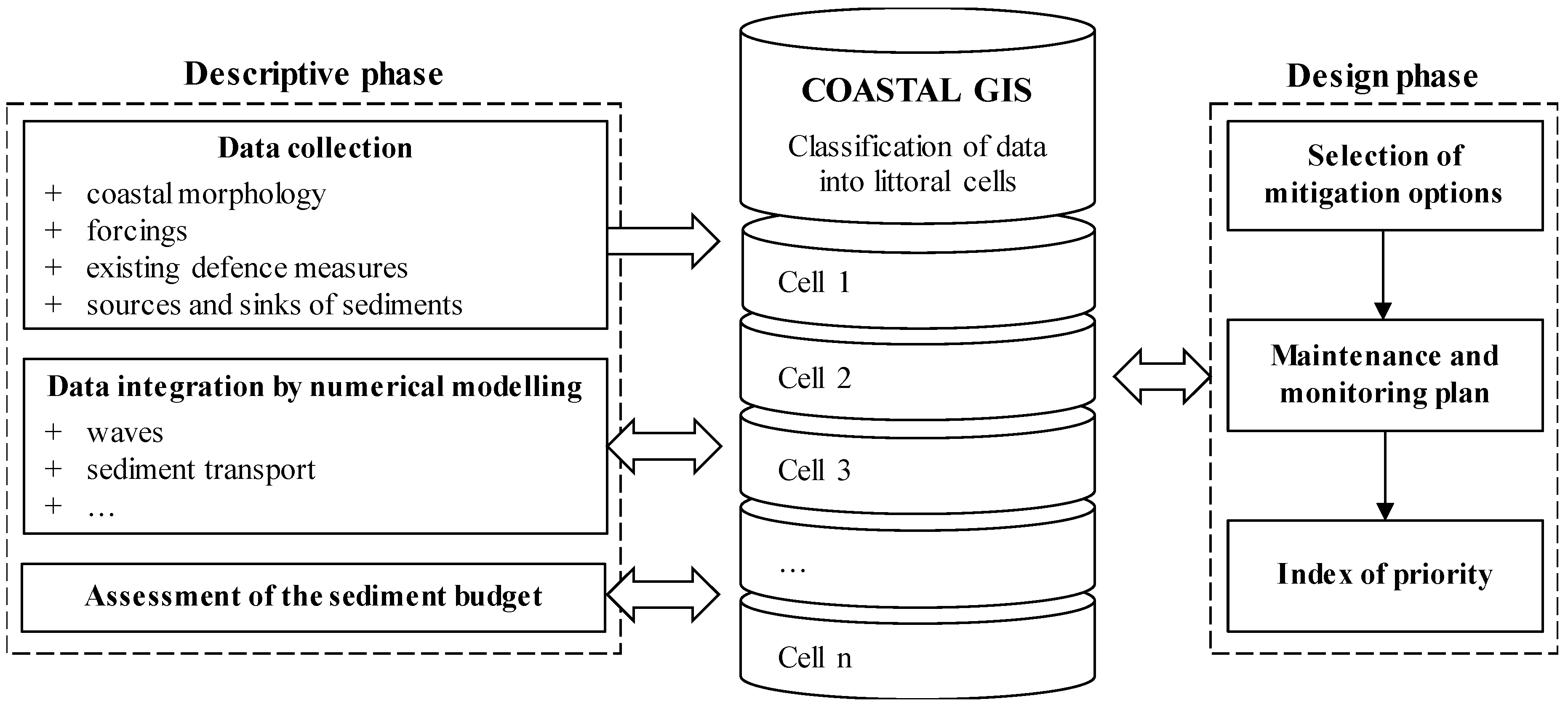
The core of the method (common to both the descriptive and design phase) involves subdividing the regional coast into littoral cells and organising all of the information and results into a single geographical information system (Coastal GIS). The concept of “sediment cells” [12,27] allows for a better understanding of sediment transport patterns. These cells are stretches of coast with similar characteristics bordered by morphological features, such as river mouths, inlets and port dams, meaning that, in the absence of major obstacles to long-shore currents, sediment is relatively free to move inside the morphological feature.
In addition, each cell is divided in half to form two semi-cells (S-C). Dividing these cells into two half (not necessarily equal in length) has practical advantages for the sediment budget balance, as the boundary conditions between them are morphologically continuous. Therefore, the long-shore sediment transport is continuous here and easy-to-compute by using wave climate and local beach orientation, and a new set of independent equations is added, allowing a more reliable assessment of the entire budget.
The Coastal GIS is a large database that is easy to access and update, and could be shared with all the stakeholders and local managers. The use of GIS for coastal management has expanded rapidly during the past decade (Bartlett and Smith [28], Wright and Bartlett [29]), and is suited to the Williams [30] approach, based on “getting”, “reordering” and “refining” the information. The collected information is suitable to be integrated within a CoastalME type framework [31].
Figure 1 shows the general structure of the proposed methodology, whereby the information gathered from both the descriptive and design phases is stored in the Coastal GIS.
2.1. Descriptive Phase
2.1.1. Data Collection and Harmonisation
Data and available measurements are collected, harmonised and stored in the Coastal GIS. Data for sediment budget analysis consist of all the variables that characterise local coastal morphology (i.e., shorelines, bathymetries, DTMs, grain size distribution, dune characterisation, subsidence, etc.), the forcing (i.e., wave, wind, tide, surge, currents, etc.) together with existing defence measures, and the sources and sinks of sediments (i.e., fluvial sediment transport, littoral sediment transport, a detailed history of past nourishments and dredgings).
Other information is required to define the constraints (e.g., areas with special legal protection or regulation, urban planning), and the value of the area in general (i.e., environmental relevance, urban and tourist pressure, local economy, cultural heritage, etc.). Additional data may be relevant to conducting flood-risk and vulnerability assessment (e.g., inland mapping, land use, emergency plans).
2.1.2. Data Integration by Numerical Modelling
Numerical models are frequently used in coastal planning, since they are useful for integrating any available information, especially on forcing, coastal flooding and sediment transport, e.g., [13,21,22,23,27,31].
Models such as ECMWF, AdCirc, Wavewatch III help provide a detailed description of the wind, currents and wave climate [32], both in terms of extremes and average values. In some cases, it is useful to statistically analyse the forcing provided by extensive databases (e.g., NOAA’s Historical Hurricane Tracks [33]).
Evaluation of the coastal flooding risk is a specific task that may be integrated using raster images included in the Coastal GIS as described in [34]. The flooding probability derived by the model is stored in form of vulnerability maps [35].
After the data collection phase, other numerical models (e.g., Mike21, X-Beach, LitPack, Gencade) are used to achieve a complete and homogeneous description of the sediment transport discharge for each of the sediment cells identified, taking into account the grain size distribution. The simulations evaluate the river sediment supply and long-shore and cross-shore sediment transport at regional level during the predefined time interval selected for the sediment balance. These data are essential for the assessment of the sediment budget and hence for the design phase.
2.1.3. Assessment of Sediment Budget
The sediment budget is essentially a mass balance equation applied to a specified time interval. It is convenient to subdivide the coastline into a number of small stretches and apply the balance to each stretch i:
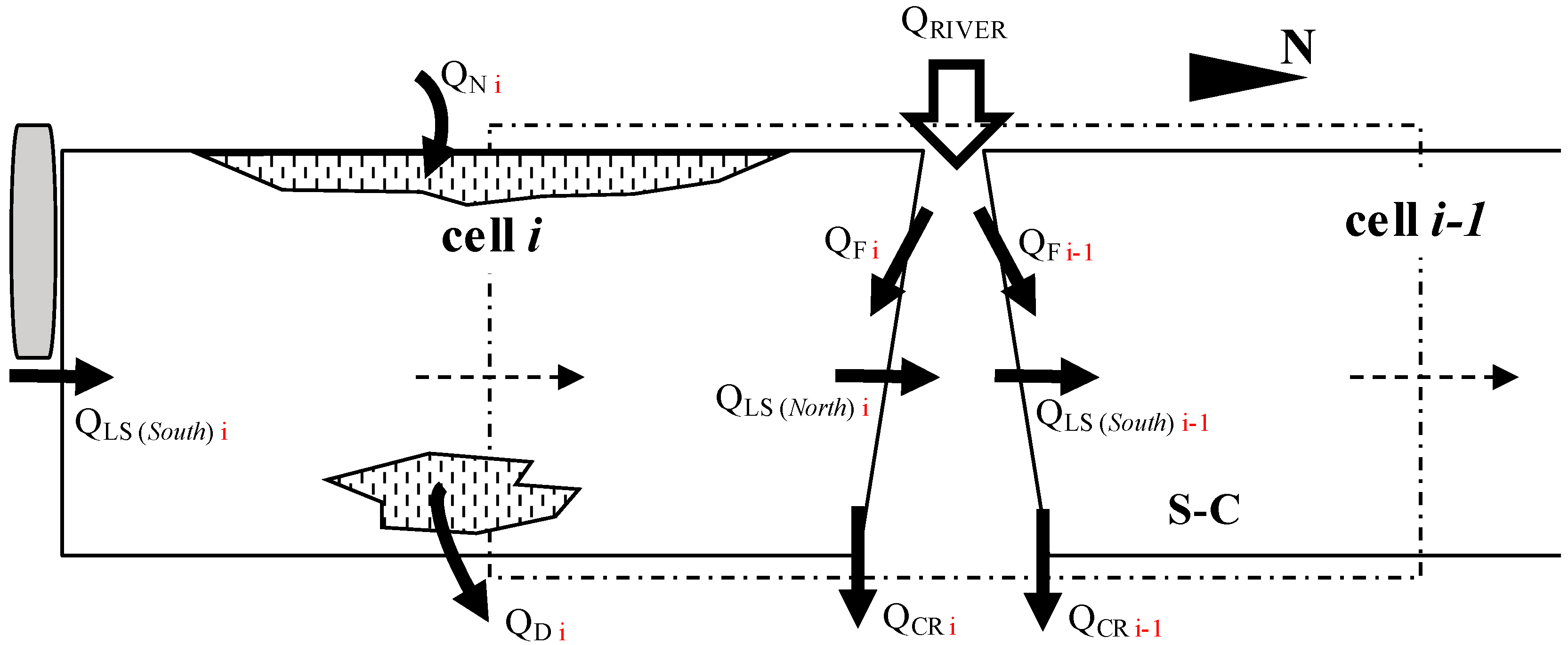
where ∂Vi is the volume of accretion or erosion estimated by a comparison of the bathymetries surveyed at the beginning and at the end of the time range , and Qi is the net sediment discharge shown in Figure 2 and given by:
where QLS is the long-shore sediment transport (North identifies the discharge at the northern boundary and South at the southern boundary in an ideal beach aligned in the North-South direction); QF is the additional river sediment supply; QCR is the cross-shore sediment transport; and QN and QD are the volumes added or subtracted due to nourishment or dredging respectively. Subsidence and sea level rise do not affect the sediment balance directly but they have the same effect as generalized erosion as they alter the marine accommodation space. In order to preserve the equilibrium profile, the accommodation space must be balanced by beach nourishment.
The balance in Equation (1) forms a system of 2n − 1 equations, where each stretch i corresponds to a semi-cell (S-C). As anticipated at the beginning of Section 2, boundary conditions between the two halves of the same littoral cell are morphologically continuous, whereas the littoral cell boundaries are placed in correspondence with morphological elements, e.g., river mouths, that can complicate the assessment of the long-shore sediment transport.
River mouths need to be considered with special attention. The inclusion of river sediment transport in the balance equations would be straightforward if the control volume extended to the two S-Cs adjacent to the mouth (i.e., the dash-dot box in Figure 2) since river supply is equivalent to nourishment. However, Equation (1) is applied to each S-C. In the adopted scheme, river sediment transport is divided and allocated to both the adjacent S-Cs, and the fine fraction losses are treated as additional off-shore sediment transport. The approach is similar to the one described by Samaras and Koutitas [36,37]. To provide a single procedure for all of the cell boundaries, the long-shore transport QLS is calculated even where the boundary is a groin, a port, a river mouth, etc. However, in presence of the latter, further calculations are required to establish QF. QF is given by the total river supply (QRIVER in Figure 2) minus the fine fraction QCR that will be transferred seaward, minus the previously calculated value of QLS. Obviously, in the trivial case of a stable river mouth, the river supply is equal to the long-shore sediment transport, and the resulting value QF is zero. It is also immediately clear that an insufficient river supply results in a negative value of QF.
The system in Equation (1) is coupled since long-shore sediment transport represents a mixed term, e.g., the QLS(South) of the Northern S-C is equal to the QLS(North) of the Southern one (dotted arrow in the middle of the cell i showed in Figure 2). It is solved using a compensation of error technique based on a matrix of uncertainties given a priori. Error compensation by least squares adjustment is obtained by solving an overdetermined system of equations based on the principle of least squares of observation residuals. It is used extensively in the disciplines of surveying, geodesy, and photogrammetry [38]. Guidelines on the evaluation of the a priori uncertainties of each term can be found, for instance, in [39]. Support of the stakeholders is essential for this phase.
2.2. Design Phase
2.2.1. Mitigation Options and Selection Criteria
Initially, based on the descriptive phase, the specific causes inducing erosion should be found, e.g., reduction of river sediment transport, increased subsidence rate, etc. Appropriate action should then be geared towards reducing these causes, e.g., providing sediment bypass in the presence of river dams and limiting extractions from the soil, etc. Similarly, reintegration of damaged structures/environmental areas shall be considered, with dune restoration being a typical measure that provides a reserve of sand in the event of storms as well as a safety against coastal flooding.
Engineering solutions for mitigation of flood and erosion risks described in [39] include both active methods, based on the reduction of the incident wave energy, such as the use of wave energy converters, floating breakwaters and artificial reefs, and passive methods, consisting of increase in overtopping resistance of dikes, improvement of resilience of breakwaters against failures, and the use of beach nourishment (possibly with innovative layout [40]) as well as tailored dredging operations. Suggestions on design optimization, optimal placement, and efficiency from an ecological perspective are outlined in [41].
Non-structural mitigation options are discussed in [42] where it is pointed out that they should be considered as part of a potential portfolio in which their combination transcends their sum, rather than standalone measures. Also, mobilization of stakeholders in the implementation process is an important issue to achieve effective results.
This sub-section puts forward the more common options and discuss their suitability for the coast of the Veneto region, which is mainly low and sandy.
Low sandy beaches can be subdivided into two categories: (1) “urbanized coasts”, which are intensely developed and have a high economic value, for which the main goal is to defend urban and tourist activities, possibly preserving a large beach; (2) “non-urbanized coasts”, natural littoral, for which the aim is to preserve the environmental value.
The proposed mitigation options follow this classification.
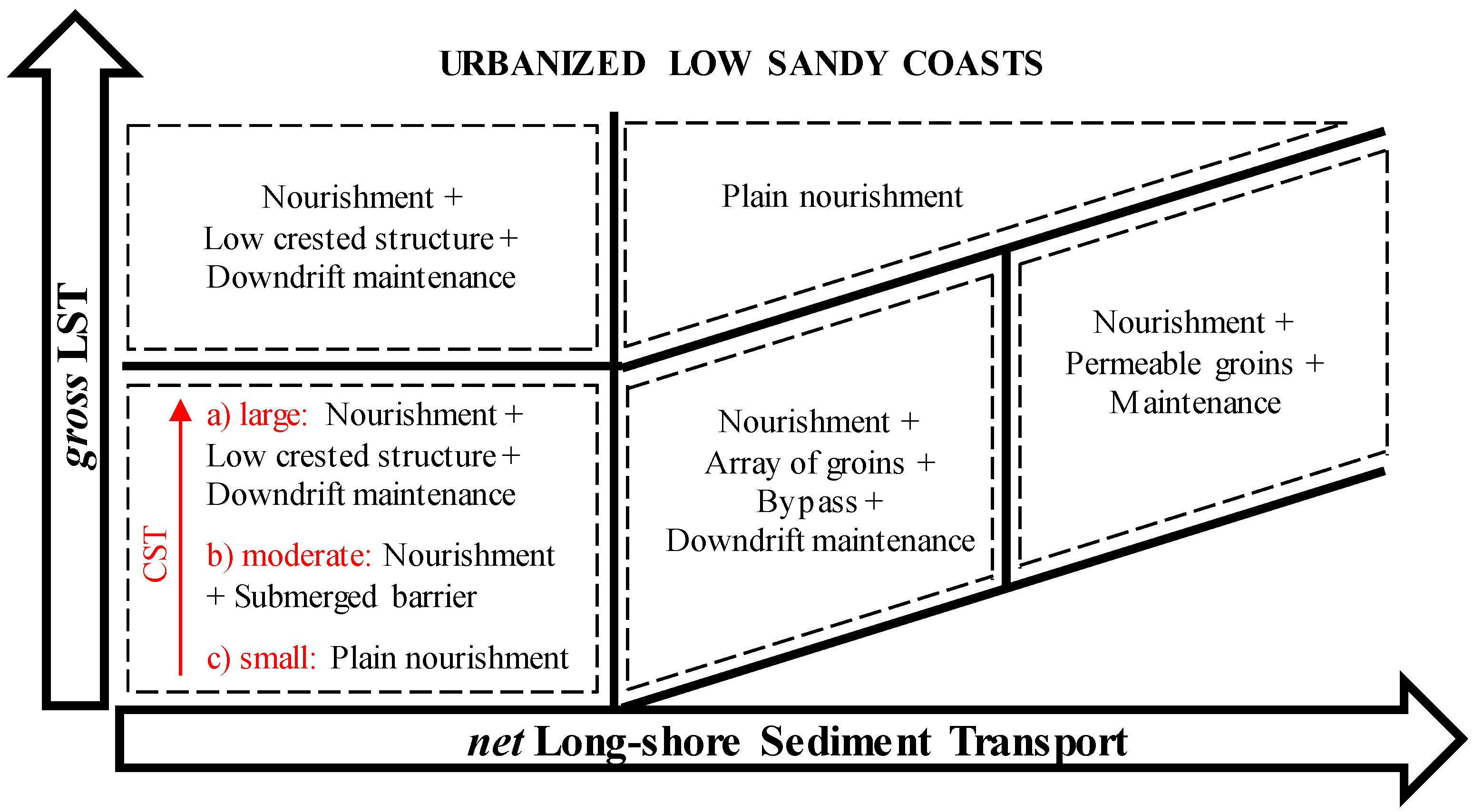
1. Urbanized low sandy coasts: The criterion is based on two main physical characteristics: the net long-shore sediment transport (net LST) and the gross long-shore sediment transport (gross LST). The rate of cross-shore sediment transport (CST) is also taken into account when LST values are low. Figure 3 shows a scheme of the guidelines for this type of coast. In all the cases, nourishment is the main strategy adopted (e.g., [43,44]), possibly together with structures (e.g., submerged barrier, low-crested structure, groins) or/and other measures (e.g., down-drift maintenance, up-drift bypass).
In particular, for very low LST (i.e., both net and gross), obstacles to LST are considered fairly ineffective at intercepting sediments. When the CST is also negligible (case “c” in Figure 3), causes of erosion are independent of coastal dynamics, and plain nourishment is the most suitable action [45]. However, when CST is appreciable (case “b” in Figure 3), the building of a submerged barrier is suggested. This structure is placed at the breaking line, deeply submerged. The expected piling up [46] and wave transmission [47] are small. It is considered effective in stabilising the cross-section profile, since breaking always occurs at the same point, and therefore the bar is stabilised, minimising the offshore CST associated with offshore bar migration [48]. For very large CST (case “a” in Figure 3), a more effective solution is required. The candidate is the low crested structure (LCS) scheme with small gaps [11], which essentially confines the sediment in the protected area, i.e., the area bordered by the shoreline, the lateral low crested groins and the offshore barrier. Note that a large piling up is expected to occur in this type of protected area, forming an obstacle to coastal dynamics and possibly resulting in some down-drift maintenance being needed [49]. The same solution is appropriate even when the gross LST is large but the net LST is small.
For large values of net and gross LST, the best solution is probably a battery of groins, as it tends to stabilise the shoreline in a saw-tooth shape and reduces LST, with benefits for the protected area [50]. However, the downdrift area (at the end of the battery of groins) must be properly maintained, and a bypass system may help reduce the sediment resource needed. In the event of extreme net LST (which only occurs with extreme gross LST), permeable groins may be considered. By reducing, but not blocking, the littoral current, the velocity differential between the velocity seaward and in the pile-groin fields is smaller than with impervious groins [51]. The primary objective of the design is to reduce the littoral current velocity to an extent that rip currents and large-scale circulations in the groin field are minimised.
When net LST is appreciable but gross LST extreme, groins are evidently not very effective [52] and do not compensate the minor CST caused by the increased wave reflection as it interacts with the structure. Plain nourishment is, therefore, the solution suggested.
In areas where the shoreline is expected to move significantly, such as in proximity of a river mouth, for which exceptional riverine sediment transport may occur, fixed structures should not be built (they may become unsuited to the modified shoreline).
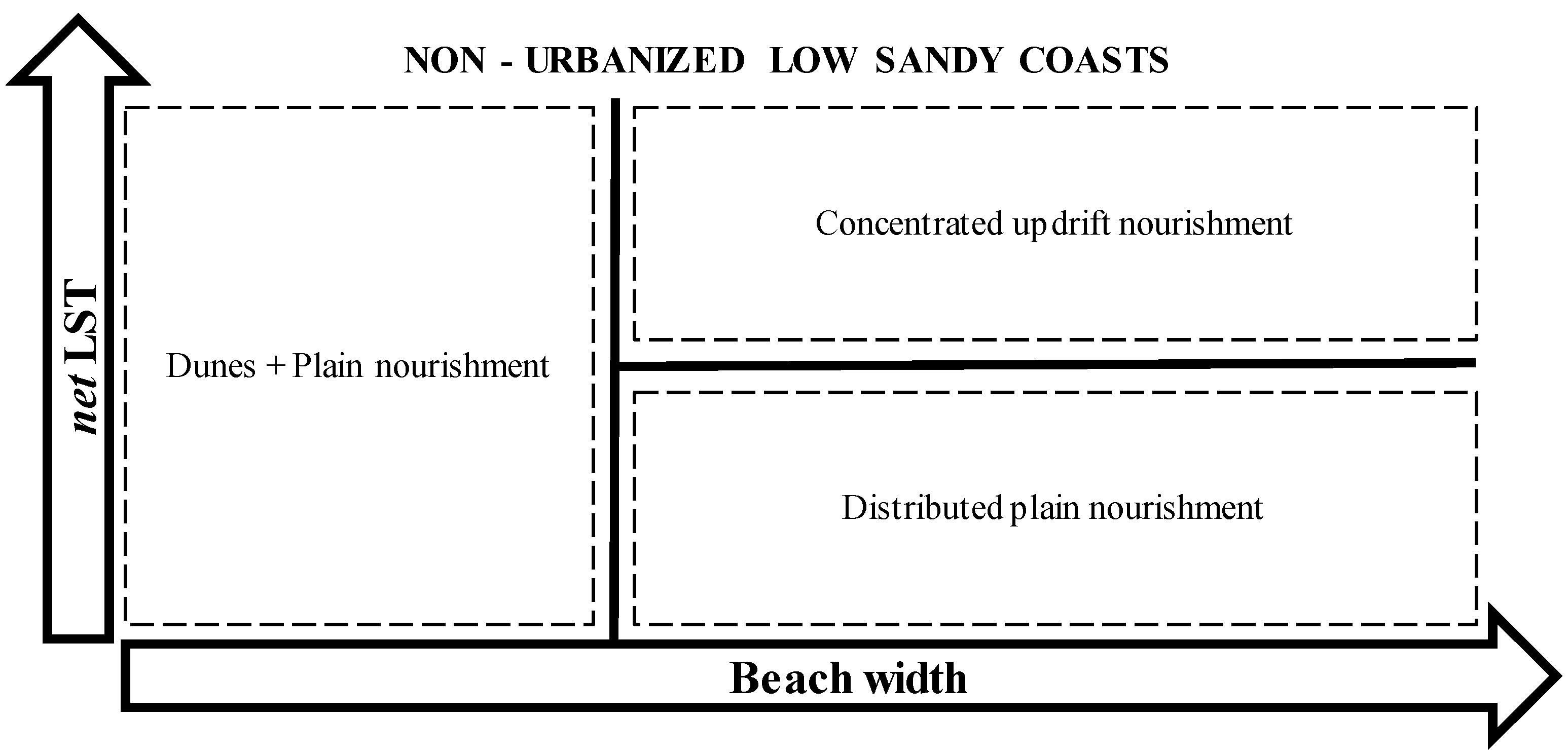
2. Non-urbanized low sandy coasts: The criterion for natural beaches (Figure 4) is based on two physical characteristics, i.e., net LST and beach width. According to Van der Nat et al. [53], who classify the degree to which coastal designs are nature-based using criteria for ecosystem-based management, the “building with nature” approach is particularly suited to this category. Three soft stabilization measures are taken into account: two measures envisage supplying sand to the beach in the form of distributed or concentrated nourishment, and one contemplates increasing sand-dune volume.
When the beach is wide and net LST large, i.e., sediment transport direction is well-defined, concentrated nourishment updrift is the least impacting solution for reducing erosion in this location, as it limits the impact of the works on a single spot and relies on littoral dynamics to redistribute sand downdrift (an extreme example is the “Sand Engine” project in the Netherlands [54]). For small net LST, the ability to redistribute nourishment is limited, so nourishment should cover the whole of the eroding coastline. Wherever the beach is narrow (i.e., may be completely eroded within a short time period), and a drastic modification of the natural environment is not viable, sand may be accumulated creating new dune systems, thus reinforcing the existing beach [55,56].
All of the aforementioned mitigation options require some degree of nourishment, making resource availability a critical issue. It is, therefore, necessary that the plan includes the location of any sediment resource along the coast, offshore and/or inland. In most cases, the sediment balance is very helpful for finding the position and size of any coastal stocks [44]. Clearly, this sediment stock makes for excellent nourishment since it belongs to the same environment and is the most economical to derive. Some care must be taken when planning the annual volumes to be dredged from these areas, and a permanent monitoring plan is necessary.
The aforementioned measures mitigate the risk of erosion. In the event of flood risk, however, strategies must be integrated with other measures [57]. Dune restoration may be considered the first candidate in order to defend the inland from marine inundation [16]. Seawalls, that induce a local erosion due to reflection, are cost-effective solutions to limit the overtopping, especially when the parapet is appropriately shaped [58,59]. LCS and other detached parallel structure, by reducing the wave energy incident directly to the coast, may have a significant impact in the reduction of run-up. Similarly, large nourishments have a very beneficial effect, both favouring energy dissipation, due to a reduced water depth, and reducing run-up, due to milder foreshore slope.
In addition to these measures, other anti-erosion and anti-flooding actions are available for both urbanized and natural coasts: managed realignment; urban planning; stabilization of river mouth (embankments to confine river discharge, plus bypass or sediment stock for updrift nourishment); lagoon dredging for environmental purposes; revetments (only where the unprotected area has no environmental and tourist interests); beach dewatering systems [60,61]; artificial reefs for habitat restoration; wave energy converter farms acting as coastal defence [62,63], seasonal interventions (e.g., sand accumulation, sand bags). It is also recommended that innovative solutions be lab-tested to ensure that they are effective in cost/benefit terms before they can be safely used on-site [16].
2.2.2. Maintenance and Monitoring Plan
The Coastal GIS should be constantly updated and all new events recorded in the database. Updates must, therefore, include results of both periodic and occasional monitoring, all the activities authorized by Regional Authorities, and an ex-post description of any coastal works carried out. It is especially important that the GIS is updated with:
- Co-ordinates and details of the methodology used to integrate information on waves, fluvial sediment transport, bathymetric profiles, etc. The plan must have a regional scale and be planned over a broad period, possibly using a common approach; it must also focus closely on the expected results.
- Results of monitoring. Each mitigation option is typically associated with a monitoring plan designed to check maintenance effectiveness and verify whether the option selected has achieved the objectives. It is highly advisable to plan an annual topo-bathymetric survey for the nourishment and additional (less frequent but specific) surveys for dunes, barriers and groins etc. These surveys should then be analysed and compared with maintenance plan predictions so that remedial action can be taken.
- Activities authorized by Coastal Authorities, such as dredging and nourishment, are to be recorded so that it is clear on which cell they were carried out, i.e., by subdividing the total dredged and nourished volumes according to the semi-cells shown in the plan. This is of great help for overall coastal management since it reduces uncertainty about total volumes.
- Any non-coastal-defence-related activities that may still contribute to the general knowledge framework.
2.2.3. Index of Priority
In addition to establishing anti-erosion and coastal flooding measures, work must be prioritized on the basis of resources and needs, and a chronological list of operations must be drawn up. The index of priority for each cell is defined as:
where the morphological vulnerability index (VM) is the sum of the erosive tendency index and the risk of coastal flooding index; the socioeconomic vulnerability index (VSE) is the sum of six indexes specifying the coast value (Table 1). The scale used for every index goes from 1 to 4 (min IP = 12, max IP = 192). The minimum and maximum value of each index are based on the lowest and highest qualitative functional response among all the analysed cells with respect to the specific aspect.
Note that the index of priority is equivalent to the “risk” defined by Benassai [64] as the product between morphological vulnerability and socioeconomic vulnerability.
3. The Venetian Littoral
3.1. Description of the Area and Assessment of Sediment Budget
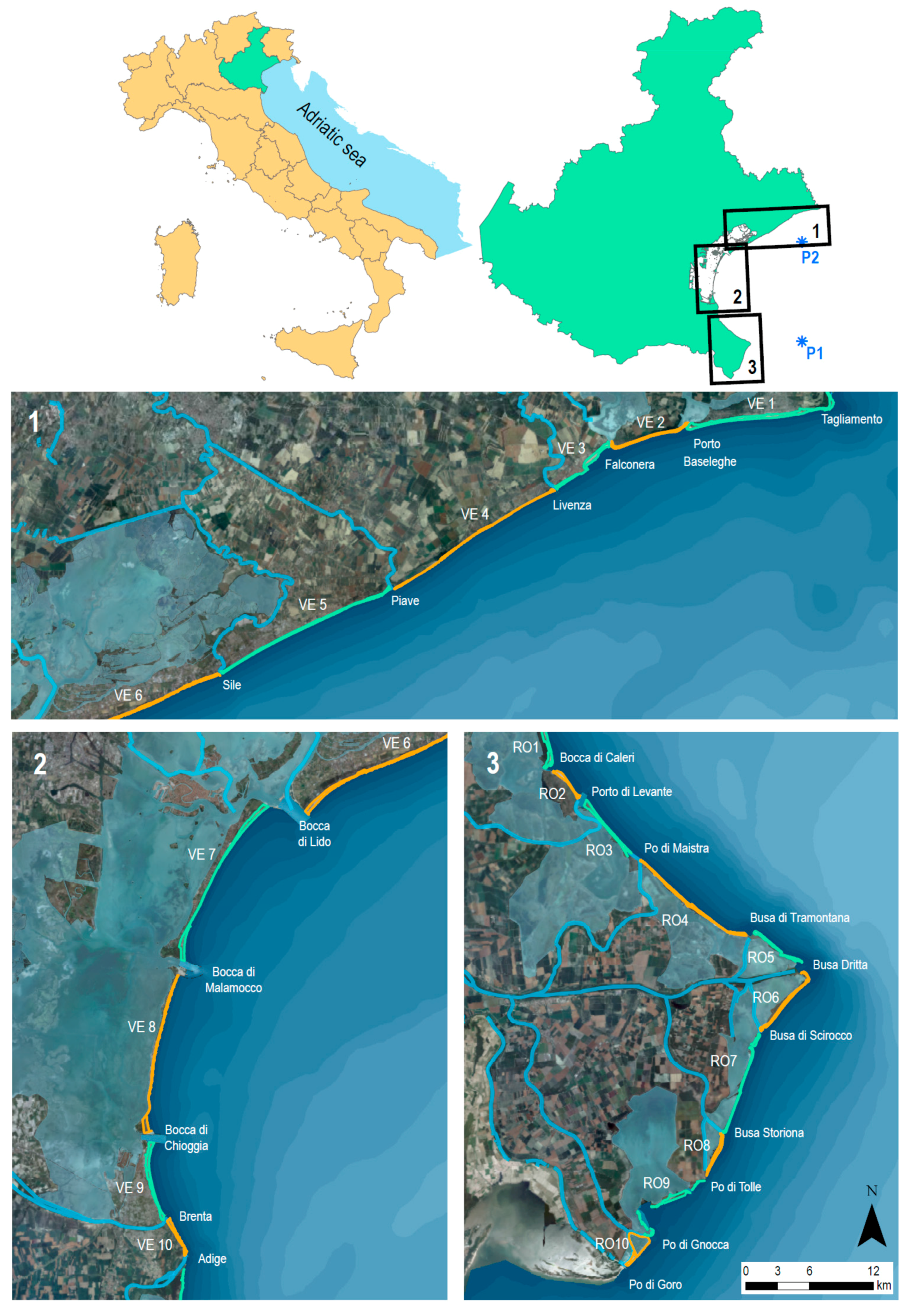
The Coastal Plan of the Veneto Region (IT) [23] (carried out according to the methods described in the previous Section) investigates the Venetian coastline (Figure 5), which is 160 km long and faces the Northern Adriatic Sea. The coastline’s borders are the mouth of the River Tagliamento to the North and the mouth of the River Po di Goro to the South. It is subdivided into two provinces and ten coastal municipalities.
The Adriatic Sea is rectangular-shaped, is about 750 km long and 200 km wide, and is connected to the Mediterranean Sea at its Southern end by the Strait of Otranto, which is about 80 km wide. Its depth is rather limited in the Northern part, where the bottom descends south-eastwards with a 1 in 1000 slope. The Adriatic coast is plagued by a combination of high waves and storm surges, which are responsible for the flooding of coastal areas, in particular, Venice and its lagoon. The highest surge was on 4 November 1966 when the sea level rose approximately 180 cm above the mean sea level (MSL) and persisted above the 100 cm mark for more than 15 h (Canestrelli [65]).
The North Adriatic Sea is characterized by two main wind (and correspondingly wave) regimes, which are primarily influenced by local orography. The prevailing winds along the Venetian coastline are the Bora and the Scirocco, which blow from the North-East and South-East respectively.
The Venetian coastline is characterized by low beaches, lagoons (i.e., Caorle, Venice and Po River Delta) and the mouths of seven rivers: the Tagliamento, Livenza, Piave, Sile, Brenta, Adige, and Po.
Along the 100 km stretch of coast from the mouth of the River Tagliamento to the Porto Caleri inlet [23] lie a vast number of areas with a high tourist value (e.g., Bibione, Caorle, Jesolo, Lido di Venezia, Sottomarina). Many of them are protected by coastal structures (e.g., groins, seawalls, breakwaters), and few are free of urban settlements (e.g., Valle Vecchia). Only a few, mainly discontinuous, dune systems can be found along the coast because they were destroyed at various times in the past.
The remaining Venetian littoral comprises the Po Delta, which covers 610 km2 and has 60 km of coast stretching from the Porto Caleri inlet to the mouth of the River Po di Goro. The active river branches of the River Po are (from North to South) Po di Maistra, Po di Pila, Po di Tolle, Po di Gnocca and Po di Goro. The coastal fringe is characterized by a sequence of low sandy and vulnerable barrier islands, beaches and spits that separate lagoons, fishing valleys, bays, tidal flats and marshes from the sea. Inland, ground elevation is almost completely below sea level (locally −2.5/−3.0 m.s.l.), and consequently the risk of coastal flooding is very high. The morphological characteristics of the Po Delta make it Italy’s largest wetland, as well as particularly unstable and very fragile when subjected to human pressure.
The Venetian coast is subdivided into 20 homogeneous littoral cells separated by inlets or the mouths of rivers (from North to South) Tagliamento, Bocca di Porto Baseleghe, Bocca di Falconera, Livenza, Piave, Sile, Bocca di Lido, Bocca di Malamocco, Bocca di Chioggia, Brenta, Adige, Bocca di Caleri, Bocca di Porto Levante, Po di Maistra, Busa Tramontana, Busa Dritta, Busa di Scirocco, Busa Storiona, Po di Tolle, Po di Gnocca, and Po di Goro. These 22 limits are shown in Figure 5 and listed in Table 2.
The plan [23] is based on the information and data available for the Venetian littoral; they comprise offshore wave characteristics, sediment grain size, topographic and bathymetric surveys over a range of time (bathymetry: 2005, 2007/2008, 2010, 2012/2014, DTM: 2008, 2012/2013), subsidence rate (1992–2000 and 2002–2010), shoreline position (1983, 2000, 2003, 2012), flooding risk maps (from 2007/60/EC directive) and a catalogue of existing shore protection structures and nourishment/dredging carried out.
Nearshore wave conditions were evaluated using the SWAN model (Simulating WAve Nearshore, [66]), developed by Delft University of Technology (NL) and based on offshore wave data. Unfortunately, a spatially refined evaluation of the offshore wave statistics obtained by oceanographic models was not available, as it is still an ongoing project. Wave information was therefore obtained by existing WAM simulations forced by data from the European Centre for Medium-Range Weather Forecasts (ECMWF) between June 1992 and December 2008, and were restricted to two points in the Northern Adriatic sea (P1: Longitude 13°00′ Latitude 45°00′, P2: Longitude 13°00′ Latitude 45°30′, wave roses in Figure 6).
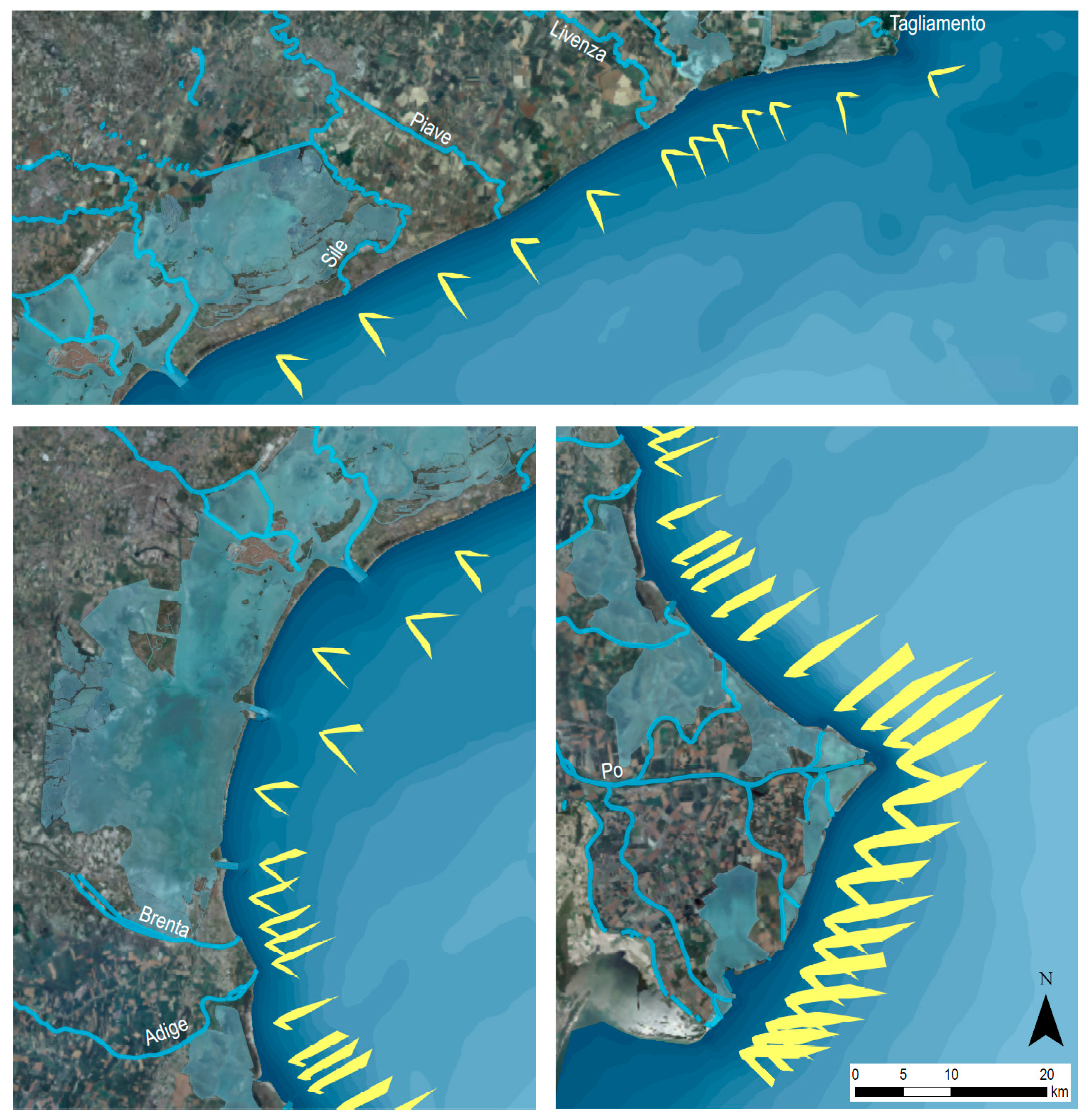
The nearshore wave climate (−10 m depth) was obtained with the SWAN model. The SWAN transforms the directional wave spectrum, which cannot be fully described by a single small plot inside a regional map. For this reason, the energy has been integrated in frequency and its directional distribution is given in the figure. For instance, Figure 7 presents the energy distribution for the point P1 and P2, whose wave climate is fully characterised by the wind rose in Figure 6. Figure 8 presents the energy distribution obtained through the SWAN model, propagating the waves from P1 and P2. The Northern part of the Venetian littoral is mainly subject to waves from the South-East, with the Scirocco blowing along the main axis of the basin and acting on a much longer fetch in this zone. Due to shoreline orientation, the Northern part of the Po Delta is exposed to the Bora, which causes high waves, although fetch is limited, with wave periods ranging between 5 and 7 s. In the Southern part of the Po Delta, sea conditions are governed by both Bora and Scirocco wind and waves. Figure 8 clearly shows that the Po Delta is characterized by larger wave energy.
Sediment surveys for the Northern Adriatic Sea have been re-organized and stored in a Coastal GIS. Table 2 shows the average sediment size for each littoral cell at different depths. In general, sediment on the Veneto coast is fine sand, with grain diameter ranging between 0.12 and 0.25 mm. As expected, grain size is coarser near the shoreline and decreases seawards. Deviations occur is some places, e.g., RO8, where rivers transport fine sediment that may deposit in the nearshore zone.
Dean [67] proposed an equilibrium profile, y = Ax2/3, giving a relationship between water depth (y) and the distance from the shoreline (x) via parameter A that, according to Hanson and Kraus [68] (A = 0.41d500.94 for d50 <0.4 mm), is a function of the median diameter d50 (mm). The formulation can be inverted to start from the bathymetric profile, so that parameter A can be adapted, and the corresponding “equilibrium diameter” dEQ can be found. The result for each littoral cell is shown in the last column of Table 2 and can be compared with actual grain size at different depths. The value of dEQ is very useful since it provides an average bed-profile shape immediately.
Assessment of the river sediment transport is complicated by the almost complete absence of systematic hydrographic surveys. Therefore, numerical models based on what little information was available were used instead. In order to evaluate river sediment discharge at the mouth, Lanzoni [69] proposed a one-dimensional numerical model using topographic surveys, the annual hydrological regime, and a medium grain size. Considering steady forcing conditions, the model estimates a “formative discharge” that produces the river topography observed and the corresponding sediment transport capacity. This approach was applied to the main rivers in the Veneto Region (Tagliamento, Piave, Brenta, Adige, and Po).
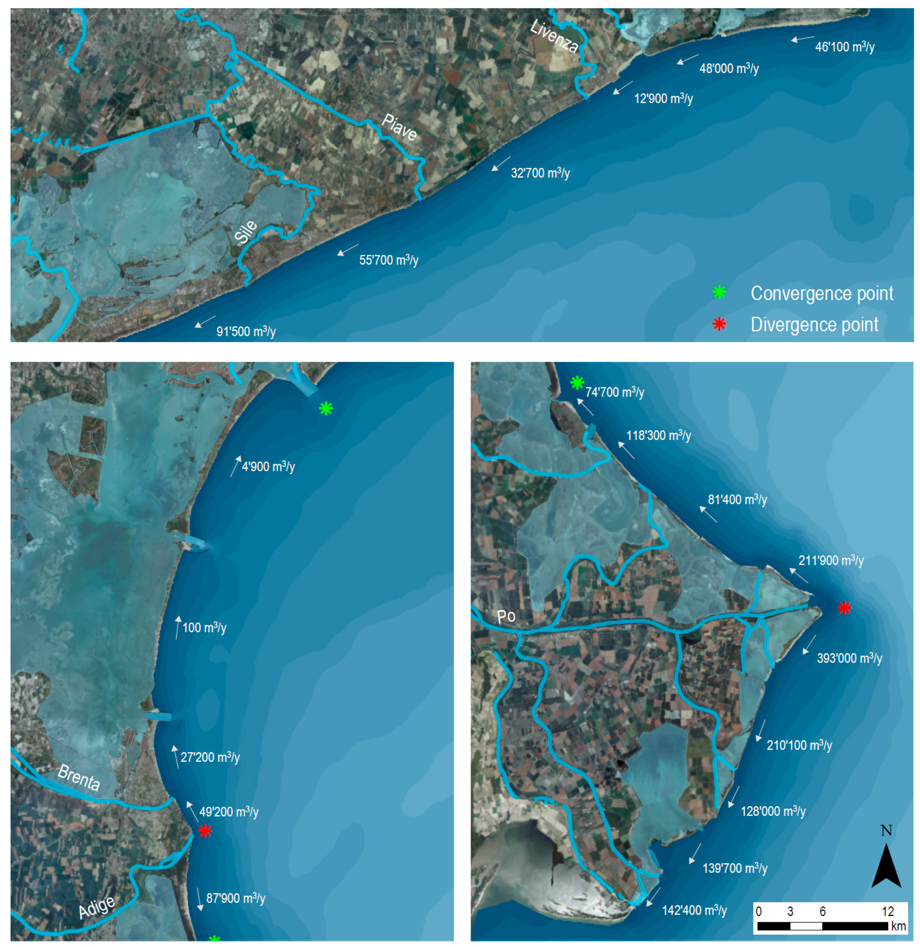
The rate of long-shore sediment transport was based on the local computation of the wave and currents for each wave state with the formula proposed by Bijker [70], following the procedure pointed out in [71], integrating across the profile and averaging. Results are shown in Figure 9 and the method is described in [23]. The spatial pattern of the simulated net transport contains divergence and convergence areas that separate areas with oppositely directed net sediment fluxes. Divergence points are located in front of the mouths of the two main rivers (Adige and Po). Convergence points are at Bocca di Lido and Bocca di Caleri. The latter, placed between cell RO1 and RO2, is a highly persistent point of convergence for net transport and thus, as observed, a deposition area (volume ~ 100,000 m3/year). The most dynamic zone is the Po Delta area, which has a symmetric morphology with a divergence net sediment transport of ~200,000 m3/year.
It was evaluated, by comparing few methods [72], that the cross-shore sediment transport QCR was heading offshore and approximately equal to 1 m3/km/year, except where the cell boundary element is a river mouth, where an additional contribution is assessed to simulate the sediment plume losses.
Subsidence along the coast is associated with natural causes related to the area’s geological history (e.g., sediment consolidation) and with anthropogenic activities, mainly fluid withdrawal. An innovative technique called Advanced Differential Interferometric SAR (A-DInSAR [73,74]) was applied in order to measure the deformation of the Earth's surface. The subsidence in the Northern part is equal to 1–2 mm/year and is mainly related to natural causes. The subsidence in the Po Delta is much larger and ranges from 3–5 mm/year, with it being linked to both natural and anthropogenic causes.
Accumulation and erosion were measured up to the depth of closure to compare successive bathymetric profiles and calculate the volume of accretion and erosion. Details and methodology are given in [75].
After the evaluation of every source term, the sediment balance for each littoral cell was calculated with Equation (1). Each homogenous littoral cell was divided into two parts in order to better appreciate the coastal processes involved. Note that the long-shore sediment transport in the middle of the cell must be the same for each semi-cell. The long-shore sediment transport at the boundary between adjacent cells may differ on account of potential depositional or erosive areas surrounding inlets or river mouths.
The balance is solved by using a compensation of error technique based on a matrix of a priori uncertainties. The accuracy of each variable is weighted with a specific coefficient and the mass unbalance for each cell is subdivided among the estimated variables forming the budget based on their weight. The final sediment budget is summarized in Table 3: 19 semi-cells (total length ~58 km) have a depositional behaviour with a volume >10,000 m3/year; 15 semi-cells (total length ~62 km) have an erosive behaviour with a volume ≤10,000 m3/year; and 6 semi-cells (total length ~19 km) are almost stable, with a volume in the range of ±10,000 m3/year.
3.2. Design Phase
Based on the sediment balance and on the criteria used to select the mitigation options (see Section 2), a coastal management proposal for every stretch of coast was carried out. For the sake of brevity, only a summary of the mitigation measures is presented here, and a detailed example of the RO1 cell is described in the next paragraph.
In the Northern zone, the goal is to “hold” the shoreline position and to protect shore-based activities using protection measures with minimum impact (e.g., avoiding seawalls, detached barriers, etc.). Management in this zone includes building a series of groins in cells VE4, VE5 and VE10 and adding large nourishments to cells VE4, VE7, VE8 and VE10 (volume = 3,650,000 m3). The global volume of sand needed for maintenance is approximately 385,000 m3/year.
A “Building with Nature” methodology is applied to the Po Delta area. Localized sand nourishment and dune reinforcement are nature-based defences that provide several ecosystem services, including flood/erosion risk mitigation and environmental conservation. The volume of sand needed for maintenance (nourishments and dunes) is approximately 145,000 m3/year.
A scheduled monitoring program was established across the entire Regional littoral in order to collect the data and information necessary.
The proposed index of prioritization was also applied to each cell to assess a chronological list of the operations based on the available resources. Figure 10 (top) shows the morphological and socioeconomic vulnerabilities along the littoral. The indexes reflect the urban essence of the area between the mouths of the rivers Tagliamento and Adige (where the main tourist activities—5,000,000 visitor/month in summer—are concentrated); the main cultural heritage sites (Venice, Caorle); and the natural essence of the Po Delta (an area with one of Italy’s highest environmental values).
Figure 10 (bottom) shows the index of priority, with the circles highlighting the 5 stretches of coast with the highest index of priority. For each stretch, the main issues are presented below.
- Coast right of the mouth of the River Tagliamento (VE1): intensive erosive processes due to reduced river supply and a system of attached breakwaters that trap the long-shore sediment transport.
- VE4 cell (Porto Santa Margherita, Duna Verde and Eraclea-Venice): erosive processes due to a decreased river sediment transport supply and the presence of reflective structures along the coast.
- Coast right of the mouth of the River Piave (VE5): intensive erosive processes due to decreased river sediment supply.
- VE 8 cell (Pellestrina-Venice): huge nourishment was conducted in the late 1990s. The effectiveness of this measure is now reduced, and intensive erosive processes are affecting this littoral. This cell is a thin barrier/island separating the Venice lagoon from the sea.
- Scardovari spit (VE9), which confined the Scardovari lagoon (in the South of the Po Delta): this vulnerable sand formation is subject to erosion processes and to episodic overwashing, which endangers the lagoon environment.
3.3. Example for RO1 Littoral Cell
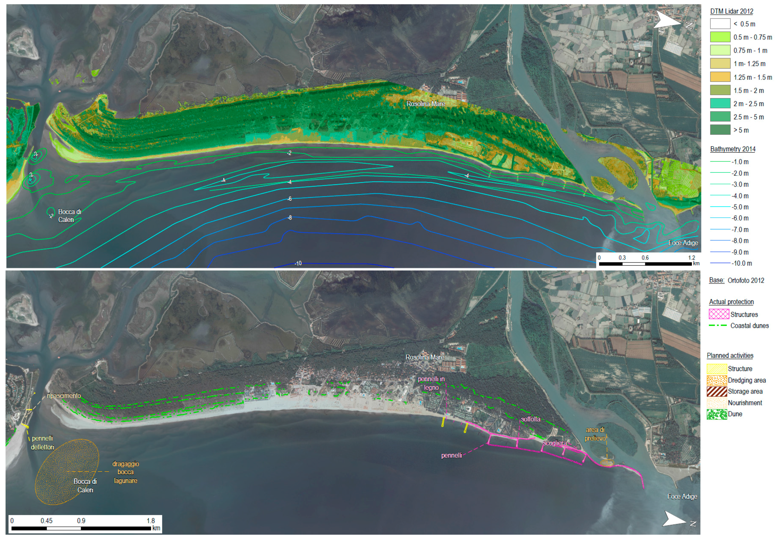
The Rosolina coastline (RO1 cell) is 8 km long and the normal shoreline direction is 80° N. The economy in the northern and central part is based mainly on tourism (1,100,000 visitors in 2016) and fishing in the backshore Caleri lagoon. The lagoon and the Southern part of the cell are major environmental areas, protected and designated as Natura 2000 sites (SCI IT3270017 and SPA IT3270023).
The cell is delimited to the North by the mouth of the River Adige which, in the final stretch, flows parallel to the beach and is confined by a weak dike that closes an old branch of the river mouth. The sediment budget analysis (Table 3) put the total fluvial sediment transport at ~265,000 m3/year, of which ~145,000 m3/year was directed toward the cell being studied (the remaining volume is directed northward toward the adjacent cell VE10). The fine sediment is lost and only ~45,000 m3/year contributes to cell advancement. Until 2007, there was a narrow beach on the sea side of the weak dike, but it has now completely disappeared, as a result of the imbalance between potential long-shore transport (~65,000 m3/year) and the actual river contribution. The crest height of this dike is very low (+1.5 m above sea level) and some waves overtop it, creating a depositional area inside the river mouth and obstructing river outflow.
Further South along the right side of the mouth of the River Adige, the beach is protected by a system of 5 groins and a detached submerged breakwater. Erosion (~13,000 m3/year) also predominates in this area due to the limited river sediment supply mentioned above, therefore an insufficient volume of 30,000 m3 is nourished every year in a bid to balance the long-shore transport directed to the Southern semi-cell (~88,000 m3/year). The interaction between nearshore hydrodynamics and the submerged barrier caused the formation of a deep channel (~3 m) in the breakwater’s seaward zone. The channel obstructs natural circulation and sand deposition from the River Adige towards the beach.
No structures were built in the southern semi-cell, as it is characterized by deposition phenomena (shoreline accretion equal to 4 m/year, volume of accretion equal to ~15,000 m3/year) since long-shore sediment transport in the Southern boundary of RO1 is reduced to ~65,000 m3/year.
The seabed appears steeper in the northern and central part than in the southern part (Caleri inlet). The −5 m isobath is 400 m from the shoreline in the northern zone, while it is 1000 m from the shoreline in the southern zone (Figure 11, top).
The Caleri inlet is a convergence point between two adjacent cells since the sand comes from the River Adige to the North and from cell RO2 to the South, making the inlet a potential dredging area (available volume ~140,000 m3/year).
The mitigation planned (Figure 11, bottom) follows on from the criteria in Figure 3. Given the large LST and the significant divergence of the LST along the northern semi-cell, the existing groins are considered appropriate, with them being reinforced and their number slightly increased. The annual nourishment volume is obtained from the sediment balance results.
Sediment resources can be derived from dredging the Caleri inlet, and it is sufficient to provide sediment elsewhere, too. A cautious dredging of only half of the forecasted annual increase in stock volume is addressed in the initial plan, and the monitoring programme will check the actual potential.
In practice, mitigation measures involve:
- Constructing a series of groins (min. 2) in the central zone in order to reduce erosion on this stretch of coast.
- Maintenance dredging the Caleri inlet (~70,000 m3/year) in order to nourish the northern and central areas and to ensure that boats can continue to navigate the lagoon inlet.
- A monitoring program.
4. Conclusions
The paper presents the method used to set up the Coastal Plan for the Venetian littoral. This method was based on a homogeneous approach at regional level consisting of a descriptive and a design phase and focused on an intensive use of a Coastal GIS database that stored both information and results, which were then organised into littoral cells and semi-cells.
The GIS also contains the sediment balance assessment obtained by analysing collected and modelled data, the accuracy of which is based on a compensation criterion. The ensuing erosion and coastal-flooding hazard, integrated with information on socioeconomic vulnerability, resulted in a priority index that highlighted the most critical areas. The information on relative sea level rise due to climate change and geodynamics are stored as they may have a relevant role for a correct design of the mitigation measures characterized by a long lifetime.
A noteworthy contribution of this paper is given in Section 2.2.1, which provides an example of a single mitigation strategy against erosion and coastal flooding for the region’s valuable urbanized and non-urbanized low sandy coasts. The consistent application of this method to the Veneto Region produced measures that were globally accepted by stakeholders, and the plan was adopted by the Regional Authorities with regional decree DGR no. 898-14/06/2016. It is conjectured that the same approach may be adopted, with due modifications, in other low sandy beaches, as well.
After a general description of the main results for the Venetian coastal plan [23], the Rosolina (RO) coastline is described in detail and provided as an example case.
Author Contributions
All the authors contributed equally in conceiving, developing and writing the article.
Acknowledgments
The Agreement between Regione Veneto and University of Padova entitled “Gestione Integrata della Zona Costiera. Progetto per lo studio ed il monitoraggio della linea di costa per la definizione degli interventi di difesa dei litorali dall’erosione nella Regione Veneto” is gratefully acknowledged.
Conflicts of Interest
The authors declare no conflict of interest.
References
- French, J.; Payo, A.; Murray, B.; Orford, J.; Eliot, M.; Cowell, P. Appropriate complexity for the prediction of coastal and estuarine geomorphic behaviour at decadal to centennial scales. Geomorphology 2016, 256, 3–16. [Google Scholar] [CrossRef]
- Haasnoot, M.; Kwakkel, J.H.; Walker, W.E.; ter Maat, J. Dynamic adaptive policy pathways: A method for crafting robust decisions for a deeply uncertain world. Glob. Environ. Chang. 2013, 23, 485–498. [Google Scholar] [CrossRef] [Green Version]
- Van Maanen, B.; Nicholls, R.J.; French, J.R.; Barkwith, A.; Bonaldo, D.; Burningham, H.; Brad Murray, A.; Payo, A.; Sutherland, J.; Thornhill, G.; et al. Simulating mesoscale coastal evolution for decadal coastal management: A new framework integrating multiple, complementary modelling approaches. Geomorphology 2016, 256, 68–80. [Google Scholar] [CrossRef]
- Hinkel, J.; Lincke, D.; Vafeidis, A.T.; Perrette, M.; Nicholls, R.J.; Tol, R.S.J.; Marzeion, B.; Fettweis, X.; Ionescu, C.; Levermann, A. Coastal flood damage and adaptation costs under 21st century sea-level rise. Proc. Natl. Acad. Sci. USA 2014, 111, 3292–3297. [Google Scholar] [CrossRef] [PubMed] [Green Version]
- Weisse, R.; Bellafiore, D.; Menéndez, M.; Méndez, F.; Nicholls, R.J.; Umgiesser, G.; Willems, P. Changing extreme sea levels along european coasts. Coast. Eng. 2014, 87, 4–14. [Google Scholar] [CrossRef]
- Toimil, A.; Losada, I.J.; Camus, P.; Díaz-Simal, P. Managing coastal erosion under climate change at the regional scale. Coast. Eng. 2017, 128, 106–122. [Google Scholar] [CrossRef]
- Stocker, T.F.; Qin, D.; Plattner, G.-K.; Tignor, M.; Allen, S.K.; Boschung, J.; Nauels, A.; Xia, Y.; Bex, V.; Midgley, P.M. IPCC Climate Change 2013: The Physical Science Basis, WG1. In The Fifth Assessment Report of the Intergovernmental Panel on Climate Change; Cambridge University Press: Cambridge, UK, 2013. [Google Scholar]
- Antonioli, F.; Anzidei, M.; Amorosi, A.; Presti, V.L.; Mastronuzzi, G.; Deiana, G.; De Falco, G.; Fontana, A.; Fontolan, G.; Lisco, S.; et al. Sea-level rise and potential drowning of the Italian coastal plains: Flooding risk scenarios for 2100. Quat. Sci. Rev. 2017, 158, 29–43. [Google Scholar] [CrossRef]
- Bezzi, A.; Pillon, S.; Martinucci, D.; Fontolan, G. Inventory and conservation assessment for the management of coastal dunes, Veneto coasts, Italy. J. Coast. Conserv. 2018, 22, 503–518. [Google Scholar] [CrossRef]
- Montanari, R.; Marasmi, C. New Tools for Coastal Management in Emilia-Romagna; Technical Report: Bologna, Italy, 2012; Available online: http://www.coastance.eu (accessed on 4 April 2018).
- Zanuttigh, B.; Martinelli, L.; Lamberti, A.; Moschella, P.; Hawkins, S.; Marzetti, S.; Ceccherelli, V.U. Environmental design of coastal defence in lido di dante, italy. Coast. Eng. 2005, 52, 1089–1125. [Google Scholar] [CrossRef]
- Doddy, P.; Ferreria, M.; Lombardo, S.; Luicus, I.; Misdorp, R.; Niesing, H.; Smallegange, M. Living with Coastal Erosion in Europe–Sediment and Space for Sustainability; Results from the Eurossion Study; European Commission Publication: Luxembourg, Luxembourg, 2004. [Google Scholar]
- Zanuttigh, B. Coastal flood protection: What perspective in a changing climate? The theseus approach. Environ. Sci. Policy 2011, 14, 845–863. [Google Scholar] [CrossRef]
- Ciavola, P.; Ferreira, O.; Haerens, P.; Van Koningsveld, M.; Armaroli, C. Storm impacts along european coastlines. Part 2: Lessons learned from the MICORE project. Environ. Sci. Policy 2011, 14, 924–933. [Google Scholar] [CrossRef]
- Armaroli, C.; Duo, E. Validation of the coastal storm risk assessment framework along the Emilia-Romagna coast. Coast. Eng. 2018, 134, 159–167. [Google Scholar] [CrossRef]
- Zanuttigh, B.; Simcic, D.; Bagli, S.; Bozzeda, F.; Pietrantoni, L.; Zagonari, F.; Hoggart, S.; Nicholls, R.J. Theseus decision support system for coastal risk management. Coast. Eng. 2014, 87, 218–239. [Google Scholar] [CrossRef]
- Torresan, S.; Critto, A.; Rizzi, J.; Zabeo, A.; Furlan, E.; Marcomini, A. Desyco: A decision support system for the regional risk assessment of climate change impacts in coastal zones. Ocean Coast. Manag. 2016, 120, 49–63. [Google Scholar] [CrossRef]
- Vafeidis, A.T.; Nicholls, R.J.; McFadden, L.; Tol, R.S.J.; Hinkel, J.; Spencer, T.; Grashoff, P.S.; Boot, G.; Klein, R.J.T. A new global coastal database for impact and vulnerability analysis to sea-level rise. J. Coast. Res. 2008, 244, 917–924. [Google Scholar] [CrossRef]
- Van Dongeren, A.; Ciavola, P.; Viavattene, C.; de Kleermaeker, S.; Martinez, G.; Ferreira, O.; Costa, C.; McCall, R. Risc-kit: Resilience-increasing strategies for coasts-toolkit. J. Coast. Res. 2014, 70, 366–371. [Google Scholar] [CrossRef]
- Stelljes, N.; Martinez, G.; McGlade, K. Introduction to the RISC-KIT web based management guide for DRR in European coastal zones. Coast. Eng. 2018, 134, 73–80. [Google Scholar] [CrossRef]
- Preti, M. Stato del litorale Emiliano-Romagnolo All’anno 2007 e Piano Decennale di Gestione; Technical Report; I quaderni di ARPA Emilia Romagna: Bologna, Italy, 2008. [Google Scholar]
- Petrillo, A.F.; Bruno, M.F.; Francioso, R.; Nobile, B.; Tomasicchio, R.; D’alessandro, F.; Di Pace, P.; Gencarelli, R. Studi Propedeutici per la Predisposizione del Piano Stralcio della Dinamica delle Coste. AdB Puglia, Politecnico di Bari, Università del Salento, Allegato 3.1 & 3.2, 2010. Available online: old.regione.puglia.it/web/files/demaniomarittimo/06__All.3.2__Strutture_per_la_difesa_delle_coste.pdf; old.regione.puglia.it/web/files/demaniomarittimo/05__All.3.1__Strutture_di_mitigazione_del_rischio.pdf (accessed on 4 April 2018).
- Ruol, P.; Martinelli, L.; Favaretto, C. Gestione Integrata della zona Costiera. Studio e Monitoraggio per la Definizione degli Interventi di Difesa dei Litorali Dall’erosione nella Regione Veneto—Linee Guida; Edizioni Libreria Progetto: Padova, Italy, 2016. [Google Scholar]
- Simeoni, U.; Corbau, C. A review of the delta Po evolution (Italy) related to climatic changes and human impacts. Geomorphology 2009, 107, 64–71. [Google Scholar] [CrossRef]
- Carbognin, L.; Teatini, P.; Tosi, L. Eustacy and land subsidence in the Venice lagoon at the beginning of the new millennium. J. Mar. Syst. 2004, 51, 345–353. [Google Scholar] [CrossRef]
- Pomaro, A.; Cavaleri, L.; Lionello, P. Climatology and trends of the Adriatic Sea wind waves: Analysis of a 37-year long instrumental data set. Int. J. Climatol. 2017, 37, 4237–4250. [Google Scholar] [CrossRef]
- California Coastal Sediment Management Workgroup. California Coastal Sediment Master Plan Status Report; Draft for Public Review and Comment; California Geological Survey: Santa Rosa, CA, USA, 2006.
- Bartlett, D.; Smith, J.L. GIS for Coastal Zone Management; CRC Press: Boca Raton, FL, USA, 2004. [Google Scholar]
- Wright, D.; Bartlett, D. Marine and Coastal Geographical Information Systems; Taylor and Francis: London, UK, 2000. [Google Scholar]
- Williams, A.; Rangel-Buitrago, N.G.; Pranzini, E.; Anfuso, G. The management of coastal erosion. Ocean Coast. Manag. 2017. [Google Scholar] [CrossRef]
- Payo, A.; Favis-Mortlock, D.; Dickson, M.; Hall, J.W.; Hurst, M.D.; Walkden, M.J.A.; Townend, I.; Ives, M.C.; Nicholls, R.J.; Ellis, M.A. Coastal Modelling Environment version 1.0: A framework for integrating landform-specific component models in order to simulate decadal to centennial morphological changes on complex coasts. Geosci. Model Dev. 2017, 10, 2715–2740. [Google Scholar] [CrossRef]
- Cavaleri, L.; Abdalla, S.; Benetazzo, L.; Bertotti, J.-R.; Bidlot, Ø.; Breivik, S.; Carniel, R.E.; Jensen, J.; Portilla-Yandun, W.E.; Rogers, A.; et al. Wave modelling in coastal and inner seas. Prog. Oceanogr. 2018. [Google Scholar] [CrossRef]
- Roy, C.; Kovordányi, R. Tropical cyclone track forecasting techniques—A review. Atmos. Res. 2012, 104, 40–69. [Google Scholar] [CrossRef]
- Favaretto, C.; Martinelli, L.; Ruol, P. Raster Based Model of Inland Coastal Flooding Propagation Using Linearized Bottom Friction and Application to a Real Case Study in Caorle, Venice (IT). In Proceedings of the Twenty-Eight International Ocean and Polar Engineering Conference (ISOPE2018), Sapporo, Japan, 10–15 June 2018. [Google Scholar]
- Martinelli, L.; Zanuttigh, B.; Corbau, C. Assessment of coastal flooding hazard along the Emilia Romagna littoral, IT. Coast. Eng. 2010, 57, 1042–1058. [Google Scholar] [CrossRef]
- Samaras, A.G.; Koutitas, C.G. The impact of catchment management on coastal morphology. The case of Fourka in Greece. J. Coast. Res. 2009, 1686–1690. [Google Scholar]
- Samaras, A.G.; Koutitas, C.G. Comparison of three longshore sediment transport rate formulae in shoreline evolution modeling near stream mouths. Ocean Eng. 2014, 92, 255–266. [Google Scholar] [CrossRef]
- Mikhail, E.D.; Gracie, G. Analysis & Adjustment of Survey Measurements; Van Nostrand Reinhold: New York, NY, USA, 1981. [Google Scholar]
- Burcharth, H.F.; Zanuttigh, B.; Andersen, T.L.; Lara, J.L.; Steendam, G.J.; Ruol, P.; Sergent, P.; Ostrowski, R.; Silva, R.; Martinelli, L.; et al. Innovative Engineering Solutions and Best Practices to Mitigate Coastal Risk. Coast. Risk Manag. Chang. Clim. 2014, 55–170. [Google Scholar] [CrossRef]
- Ruol, P.; Martinelli, L.; Favaretto, C.; Scroccaro, D. Innovative Sand Groin Beach Nourishment with Environmental, Defense and Recreational Purposes. In Proceedings of the Twenty-Eight International ocean and polar engineering conference (ISOPE2018), Sapporo, Japan, 10–15 June 2018. [Google Scholar]
- Hoggart, S.; Hawkins, S.J.; Bohn, K.; Airoldi, L.; van Belzen, J.; Bichot, A.; Bilton, D.T.; Bouma, T.J.; Colangelo, M.A.; Davies, A.J.; et al. Ecological approaches to coastal risk mitigation. Coast. Risk Manag. Chang. Clim. 2015, 171–236. [Google Scholar] [CrossRef]
- Vanderlinden, J.P.; Baztan, J.; Coates, T.; Dávila, O.G.; Hissel, F.; Kane, I.O.; Koundouri, P.; McFadden, L.; Parker, D.; Penning-Rowsell, E.; et al. Nonstructural approaches to coastal risk mitigations. Coast. Risk Manag. Chang. Clim. 2015, 237–274. [Google Scholar] [CrossRef]
- Bergillos, R.J.; López-Ruiz, A.; Principal-Gómez, D.; Ortega-Sánchez, M. An integrated methodology to forecast the efficiency of nourishment strategies in eroding deltas. Sci. Total Environ. 2018, 613, 1175–1184. [Google Scholar] [CrossRef] [PubMed]
- Stronkhorst, J.; Huisman, B.; Giardino, A.; Santinelli, G.; Santos, F.D. Sand nourishment strategies to mitigate coastal erosion and sea level rise at the coasts of Holland (The Netherlands) and Aveiro (Portugal) in the 21st century. Ocean Coast. Manag. 2018, 156, 266–276. [Google Scholar] [CrossRef]
- Dean, R.G. Beach Nourishment: Theory and Practice; World Scientific Publishing Company: Toh Tuck Link, Singapore, 2003. [Google Scholar]
- Zanuttigh, B.; Martinelli, L.; Lamberti, A. Wave overtopping and piling-up at permeable low crested structures. Coast. Eng. 2008, 55, 484–498. [Google Scholar] [CrossRef]
- Buccino, M.; Calabrese, M. Conceptual approach for prediction of wave transmission at low-crested breakwaters. J. Waterw. Port Coast. Ocean Eng. 2007, 133, 213–224. [Google Scholar] [CrossRef]
- Martinelli, L.; Zanuttigh, B.; De Nigris, N.; Preti, M. Sand bag barriers for coastal protection along the emilia romagna littoral, northern adriatic sea, Italy. Geotext. Geomembr. 2011, 29, 370–380. [Google Scholar] [CrossRef]
- Hawkins, S.J.; Burcharth, H.F.; Zanuttigh, B.; Lamberti, A. Environmental Design Guidelines for Low Crested Coastal Structures; Elsevier: Oxford, UK, 2010. [Google Scholar]
- Basco, D.R.; Pope, J. Groin Functional Design Guidance from the Coastal Engineering Manual; Coastal Education & Research Foundation, Inc.: Collier County, FL, USA, 2004; pp. 121–130. [Google Scholar]
- Raudkivi, A.J. Permeable pile groins. J. Waterw. Port Coast Ocean Eng. 1996, 122, 267–272. [Google Scholar] [CrossRef]
- Kristensen, S.E.; Drønen, N.; Deigaard, R.; Fredsoe, J. Impact of groyne fields on the littoral drift: A hybrid morphological modelling study. Coast. Eng. 2016, 111, 13–22. [Google Scholar] [CrossRef] [Green Version]
- Van der Nat, A.; Vellinga, P.; Leemans, R.; Van Slobbe, E. Ranking coastal flood protection designs from engineered to nature-based. Ecol. Eng. 2016, 87, 80–90. [Google Scholar] [CrossRef]
- Stive, M.J.F.; de Schipper, M.A.; Luijendijk, A.P.; Aarninkhof, S.G.J.; van Gelder-Maas, C.; van Thiel de Vries, J.S.M.; de Vries, S.; Henriquez, M.; Marx, S.; Ranasinghe, R. A new alternative to saving our beaches from sea-level rise: The sand engine. J. Coast. Res. 2013, 290, 1001–1008. [Google Scholar] [CrossRef]
- Hanley, M.E.; Hoggart, S.P.G.; Simmonds, D.J.; Bichot, A.; Colangelo, M.A.; Bozzeda, F.; Heurtefeux, H.; Ondiviela, B.; Ostrowski, R.; Recio, M.; et al. Shifting sands? coastal protection by sand banks, beaches and dunes. Coast. Eng. 2014, 87, 136–146. [Google Scholar] [CrossRef]
- Gracia, C.A.; Rangel-Buitrago, N.; Oakley, J.A.; Williams, A. Use of ecosystems in coastal erosion management. Ocean Coast. Manag. 2018, 156, 277–289. [Google Scholar] [CrossRef]
- Villatoro, M.; Silva, R.; Méndez, F.J.; Zanuttigh, B.; Pan, S.; Trifonova, E.; Losada, I.J.; Izaguirre, C.; Simmonds, D.; Reeve, D.E.; et al. An approach to assess flooding and erosion risk for open beaches in a changing climate. Coast. Eng. 2014, 87, 50–76. [Google Scholar] [CrossRef]
- McCabe, M.V.; Stansby, P.K.; Apsley, D.D. Random wave runup and overtopping a steep sea wall: Shallow-water and boussinesq modelling with generalised breaking and wall impact algorithms validated against laboratory and field measurements. Coast. Eng. 2013, 74, 33–49. [Google Scholar] [CrossRef]
- Castellino, M.; Sammarco, P.; Romano, A.; Martinelli, L.; Ruol, P.; Franco, L.; De Girolamo, P. Large impulsive forces on recurved parapets under non-breaking waves. A numerical study. Coast. Eng. 2018, 136, 1–15. [Google Scholar] [CrossRef]
- Damiani, L.; Aristodemo, F.; Saponieri, A.; Verbeni, B.; Veltri, P.; Vicinanza, D. Full-scale experiments on a beach drainage system: Hydrodynamic effects inside beach. J. Hydraul. Res. 2011, 49, 44–54. [Google Scholar] [CrossRef]
- Damiani, L.; Vicinanza, D.; Aristodemo, F.; Saponieri, A.; Corvaro, S. Experimental investigation on wave set-up and nearshore velocity field in presence of a BDS. J. Coast. Res. 2011, SI 64, 55–59. [Google Scholar]
- Ruol, P.; Zanuttigh, B.; Martinelli, L.; Kofoed, P.; Frigaard, P. Near-shore floating wave energy converters: Applications for coastal protection. Coast. Eng. Proc. 2011, 1. [Google Scholar] [CrossRef]
- Mendoza, E.; Silva, R.; Zanuttigh, B.; Angelelli, E.; Lykke Andersen, T.; Martinelli, L.; Nørgaard, J.Q.H.; Ruol, P. Beach response to wave energy converter farms acting as coastal defence. Coast. Eng. 2014, 87, 97–111. [Google Scholar] [CrossRef]
- Benassai, G.; Chirico, F.; Corsini, S. Una metodologia sperimentale per la definizione del rischio da inondazione costiera. Stud. Costieri 2009, 16, 51–72. [Google Scholar]
- Canestrelli, P.; Mandich, M.; Pirazzoli, P.A.; Tomasin, A. Wind, depression and seiches: Tidal perturbations in Venice (1951–2000). Centro Previsioni e Segnalazioni Maree. Comune Venezia 2001, 1–104. [Google Scholar]
- Booij, N.; Ris, R.C.; Holthuijsen, L.H. A third-generation wave model for coastal regions: 1. Model description and validation. J. Geophys. Res. Ocean. 1999, 104, 7649–7666. [Google Scholar] [CrossRef] [Green Version]
- Dean, R.G. Equilibrium Beach Profiles: US Atlantic and Gulf Coasts; Department of Civil Engineering and College of Marine Studies; Technical Report 12; University of Delaware: Newark, DE, USA, 1977. [Google Scholar]
- Hanson, H.; Kraus, N.C. GENESIS: Generalized Model for Simulating Shoreline Change; Report 1. Technical Reference; Technical Report CERC-89-19; Coastal Engineering Research Center: Vicksburg, MS, USA, 1989. [Google Scholar]
- Lanzoni, S.; Luchi, R.; Bolla Pittaluga, M. Modeling the morphodynamic equilibrium of an intermediate reach of the po river (Italy). Adv. Water Resour. 2015, 81, 95–102. [Google Scholar] [CrossRef]
- Bijker, E.W. Some Considerations about Scales for Coastal Models with Movable Bed. Ph.D. Thesis, Delft Hydraulics Laboratory Publication, Delft, The Netherlands, 1967. [Google Scholar]
- Bayram, A.; Larson, M.; Miller, H.C.; Kraus, N.C. Cross-shore distribution of longshore sediment transport: Comparison between predictive formulas and field measurements. Coast. Eng. 2001, 44, 79–99. [Google Scholar] [CrossRef]
- Schoonees, J.S.; Theron, A.K. Evaluation of 10 cross-shore sediment transport/morphological models. Oceanogr. Lit. Rev. 1996, 2, 136. [Google Scholar] [CrossRef]
- Ferretti, A.; Prati, C.; Rocca, F. Permanent scatterers in sar interferometry. IEEE Trans. Geosci. Remote. Sens. 2001, 39, 8–20. [Google Scholar] [CrossRef]
- Lanari, R.; Mora, O.; Manunta, M.; Mallorqui, J.J.; Berardino, P.; Sansosti, E. A small-baseline approach for investigating deformations on full-resolution differential sar interferograms. IEEE Trans. Geosci. Remote Sens. 2004, 42, 1377–1386. [Google Scholar] [CrossRef]
- Fontolan, G.; Bezzi, A.; Martinucci, D.; Pillon, S.; Popesso, C.; Rizzetto, F. Sediment budget and management of the Veneto beaches, Italy: An application of the modified Littoral Cells Management System (SICELL). Proceedings of Coastal and Maritime Mediterranean Conference, Ferrare, Italy, 25–27 November 2015. [Google Scholar]
Figure 1.
Breakdown of coastal plan activities. The Coastal GIS includes both data (measured or computed) gathered in the descriptive phase and the results following the design phase.
Figure 1.
Breakdown of coastal plan activities. The Coastal GIS includes both data (measured or computed) gathered in the descriptive phase and the results following the design phase.

Figure 2.
Sediment balance diagram. Littoral cells are limited by morphological features (continuous line). The inclusion of river sediment transport in the balance equations would be straightforward if the cell control volume extended to the dash-dot box.
Figure 2.
Sediment balance diagram. Littoral cells are limited by morphological features (continuous line). The inclusion of river sediment transport in the balance equations would be straightforward if the cell control volume extended to the dash-dot box.

Figure 3.
Guidelines for erosion mitigation strategies (div(LST) = divergence of long-shore sediment transport, CST = cross-shore sediment transport) for urbanized low sandy coasts.
Figure 3.
Guidelines for erosion mitigation strategies (div(LST) = divergence of long-shore sediment transport, CST = cross-shore sediment transport) for urbanized low sandy coasts.

Figure 4.
Guidelines for erosion mitigation strategies (div (LST) = divergence of long-shore sediment transport) for non-urbanized low sandy coasts.
Figure 4.
Guidelines for erosion mitigation strategies (div (LST) = divergence of long-shore sediment transport) for non-urbanized low sandy coasts.

Figure 5.
Venetian littoral and its subdivision into coastal cells.

Figure 6.
Offshore wave climate in the Northern Adriatic Sea: point P1 (left), point P2 (right).

Figure 7.
Offshore Energy polar plot relative to point P1 (left), point P2 (right) summarising the wave rose in Figure 6.
Figure 7.
Offshore Energy polar plot relative to point P1 (left), point P2 (right) summarising the wave rose in Figure 6.

Figure 8.
Nearshore wave climate (energy polar plot) for the Venetian littoral. The scale of the energy plot is common to the three images, allowing a qualitative comparison.
Figure 8.
Nearshore wave climate (energy polar plot) for the Venetian littoral. The scale of the energy plot is common to the three images, allowing a qualitative comparison.

Figure 9.
Long-shore sediment transport for the Venetian littoral.

Figure 10.
Vulnerability and index of priority.

Figure 11.
Topo-bathymetry (top) and adopted mitigation for the RO1 cell.


Table 1.
Description of terms VM and VSE in Equation (3).
| Morphological Vulnerability (VM) | Socioeconomic Vulnerability (VSE) |
|---|---|
| Erosive Trend Coastal Flooding Risk | Value of coastal defence action (frequency and financial investments) Environmental relevance (presence of natural areas, Natura2000 sites, etc.) Tourist pressure (number of tourist/year, bathing facilities, tourist facilities, etc.) Urbanization (presence of cities, type of inland, etc.) Production activities (fishing, mussel/clam farming, etc.) Cultural heritage (monuments, archaeological sites, etc.) |
Table 2.
Littoral cell boundary, sediment diameter (d50, mm) sampled at different depths and evaluated with the Dean rule (dEQ, mm).
Table 2.
Littoral cell boundary, sediment diameter (d50, mm) sampled at different depths and evaluated with the Dean rule (dEQ, mm).
| Cell | North Bound | South Bound | d50 0 m/−2 m | d50 −2 m/−4 m | d50 −4 m/−6 m | d50 <−6 m | dEQ |
|---|---|---|---|---|---|---|---|
| VE1 | Tagliamento | Porto Baseleghe | 0.323 | - | - | - | 0.14 |
| VE2 | Porto Baseleghe | Falconera | 0.173 | - | - | - | 0.13 |
| VE3 | Falconera | Livenza | 0.175 | 0.235 | 0.118 | - | 0.16 |
| VE4 | Livenza | Piave | 0.205 | 0.173 | 0.143 | - | 0.16 |
| VE5 | Piave | Sile | 0.153 | 0.268 | 0.118 | - | 0.15 |
| VE6 | Sile | Bocca di Lido | - | 0.235 | 0.213 | - | 0.14 |
| VE7 | Bocca di Lido | Bocca di Malamocco | 0.181 | - | 0.186 | - | 0.12 |
| VE8 | Bocca di Malamocco | Bocca di Chioggia | - | - | - | - | 0.20 |
| VE9 | Bocca di Chioggia | Foce Brenta | - | 0.144 | 0.168 | - | 0.15 |
| VE10 | Brenta | Adige | - | - | - | - | 0.24 |
| RO1 | Adige | Bocca di Caleri | - | 0.190 | 0.191 | 0.129 | 0.18 |
| RO2 | Bocca di Caleri | Porto di Levante | - | 0.139 | 0.126 | 0.110 | 0.11 |
| RO3 | Porto di Levante | Po di Maistra | - | 0.143 | 0.185 | 0.142 | 0.11 |
| RO4 | Po di Maistra | Busa di Tramontana | - | 0.173 | 0.208 | 0.133 | 0.13 |
| RO5 | Busa di Tramontana | Busa Dritta | - | 0.234 | 0.230 | 0.101 | 0.17 |
| RO6 | Busa Dritta | Busa di Scirocco | - | 0.273 | 0.258 | 0.207 | 0.17 |
| RO7 | Busa di Scirocco | Busa Storiona | - | 0.167 | 0.148 | 0.132 | 0.17 |
| RO8 | Busa Storiona | Po di Tolle | - | 0.068 | 0.197 | 0.100 | 0.15 |
| RO9 | Po di Tolle | Po di Gnocca | - | 0.144 | 0.146 | - | 0.10 |
| RO10 | Po di Gnocca | Po di Goro | - | - | - | - | 0.13 |
Table 3.
Sediment balance (thousand m3/year).
| Cell | Part | QLS (1) Long-shore | QLS (2) Long-shore | QCR Cross-shore | QF Fluvial | QN Nourished | QD Dredged | ∂V |
|---|---|---|---|---|---|---|---|---|
| VE1 | N | −30.9 | −46.1 | 22.7 | 11.0 | 51.0 | 49.0 | −24.9 |
| VE1 | S | −46.1 | −48.9 | 7.1 | 65.9 | - | - | 55.9 |
| VE2 | N | −67.9 | −48.0 | 4.4 | - | - | - | 15.6 |
| VE2 | S | −48.0 | −36.4 | 3.0 | - | 22.8 | 17.2 | 14.1 |
| VE3 | N | −20.3 | −12.9 | 4.6 | - | 24.0 | 0.0 | 26.9 |
| VE3 | S | −12.9 | −10.0 | 3.8 | - | 22.4 | 5.1 | 16.3 |
| VE4 | N | −10.0 | −32.7 | 8.9 | - | 64.4 | - | 32.8 |
| VE4 | S | −32.7 | −57.3 | 79.8 | 13.0 | 29.9 | - | −61.5 |
| VE5 | N | −62.6 | −55.7 | 183.7 | 117.3 | 40.0 | 40.0 | −59.6 |
| VE5 | S | −55.7 | −91.2 | 19.7 | - | 35.6 | - | −19.6 |
| VE6 | N | −75.6 | −91.5 | 22.1 | - | 20.1 | - | −17.9 |
| VE6 | S | −91.5 | −24.3 | 17.2 | - | - | 20.2 | 29.8 |
| VE7 | N | −0.7 | 4.9 | 9.3 | - | 10.0 | - | 6.4 |
| VE7 | S | 4.9 | 2.1 | 9.9 | - | 10.0 | - | −2.7 |
| VE8 | N | 2.0 | 0.1 | 18.8 | - | - | - | −20.7 |
| VE8 | S | 0.1 | 2.3 | 18.0 | - | - | - | −15.8 |
| VE9 | N | −0.6 | 27.2 | 4.6 | - | - | - | 23.2 |
| VE9 | S | 27.2 | 16.2 | 48.0 | 19.8 | 39.9 | 20.0 | −19.3 |
| VE10 | N | 48.2 | 49.2 | 43.6 | 8.3 | 34.9 | 20.0 | −19.3 |
| VE10 | S | 49.2 | 58.0 | 93.2 | 62.5 | 35.0 | - | 13.1 |
| RO1 | N | −64.9 | −87.9 | 100.1 | 80.4 | 30.0 | - | −12.6 |
| RO1 | S | −87.9 | −65.0 | 6.0 | - | - | - | 16.8 |
| RO2 | N | 79.2 | 74.7 | 2.8 | - | - | - | −7.2 |
| RO2 | S | 74.7 | 62.9 | 3.6 | - | - | - | −15.4 |
| RO3 | N | 75.4 | 118.3 | 7.9 | - | - | - | 35.0 |
| RO3 | S | 118.3 | 86.3 | 31.6 | 60.1 | - | - | −3.5 |
| RO4 | N | 86.3 | 81.4 | 39.1 | 71.4 | - | - | 27.4 |
| RO4 | S | 81.4 | 207.6 | 20.8 | - | - | 59.3 | 46.1 |
| RO5 | N | 195.6 | 211.9 | 6.7 | - | - | - | 9.6 |
| RO5 | S | 211.9 | 359.8 | 368.8 | 240.4 | - | - | 19.4 |
| RO6 | N | −409.6 | −393.0 | 370.5 | 534.0 | - | - | 180.2 |
| RO6 | S | −393.0 | −305.3 | 8.7 | - | - | - | 78.9 |
| RO7 | N | −234.7 | −210.1 | 9.4 | - | - | - | 15.2 |
| RO7 | S | −210.1 | −252.5 | 9.0 | - | - | - | −51.3 |
| RO8 | N | −230.5 | −128.0 | 6.2 | - | - | - | 96.3 |
| RO8 | S | −128.0 | −103.5 | 96.9 | 99.1 | - | - | 26.8 |
| RO9 | N | −172.9 | −139.7 | 97.3 | 64.4 | - | - | 0.3 |
| RO9 | S | −139.7 | −190.5 | 78.6 | 106.2 | - | - | −23.2 |
| RO10 | N | −95.8 | −142.4 | 5.0 | - | - | - | −51.6 |
| RO10 | S | −142.4 | −155.5 | 119.5 | 120.8 | - | - | −11.8 |
© 2018 by the authors. Licensee MDPI, Basel, Switzerland. This article is an open access article distributed under the terms and conditions of the Creative Commons Attribution (CC BY) license (http://creativecommons.org/licenses/by/4.0/).
Share and Cite
MDPI and ACS Style
Ruol, P.; Martinelli, L.; Favaretto, C. Vulnerability Analysis of the Venetian Littoral and Adopted Mitigation Strategy. Water 2018, 10, 984. https://doi.org/10.3390/w10080984
AMA Style
Ruol P, Martinelli L, Favaretto C. Vulnerability Analysis of the Venetian Littoral and Adopted Mitigation Strategy. Water. 2018; 10(8):984. https://doi.org/10.3390/w10080984
Chicago/Turabian StyleRuol, Piero, Luca Martinelli, and Chiara Favaretto. 2018. "Vulnerability Analysis of the Venetian Littoral and Adopted Mitigation Strategy" Water 10, no. 8: 984. https://doi.org/10.3390/w10080984
Note that from the first issue of 2016, this journal uses article numbers instead of page numbers. See further details here.